Deep Learning is highly empirical domain which majorly focusses on fine tuning the various parameters. The choice of these parameters defines the accuracy of model. So, it becomes important to choose such parameters wisely. Choosing the parameters based on intuition might not work every time which can degrade the performance of the model drastically. Also, a considerable amount of time and effort will go in vain while selecting the values of parameters based on intuition. So, the methodological approach should be followed to select the optimal values of parameters to maximize the accuracy of the model.
There is an n number of parameters which needs to be fine-tuned. Some of them are:
Number of layers
Number of hidden units
Choice of activation function such as sigmoid, tanh or rectified linear unit
Choice of optimization algorithms such as Gradient Descent, Adam optimization.
Regularization Techniques such as L2 regularization or L1 regularization
Network architecture such as Recurrent Neural Network(RNN), Convolutional Neural Network(CNN)
Collect more data.
Before deep diving directly into bias-variance trade off, let us discuss systematic approach to handle the Machine Learning problem.
The very first step to handle the machine learning problem is:
Set the correct distribution of train set, cross-validation or development set and test set.
Select the correct the evaluation metric depending on the problem statement.
Let’s talk about above mentioned points in detail:
Data set is divided into train set, cross validation set often called as development sets and test set. Generally, ratio of 60-20-20 is followed i.e. 60% of data is used to train the model, 20% data for cross validating the model to fine tune the parameters and 20% data to test the accuracy of model on unbiased data set. One most important thing to keep in mind here is not to follow the general rule blindly. The distribution of data into train set, development set and test set majorly depend on the size of data. For instance, if observations in data set is as high as 1000000. Then 90-5-5 ratio or even 98-1-1 ratio works far better than usual 60-20-20 rule. This is because all deep learning models has hunger for data. Using 60-20-20 distribution in such scenario would waste the large chunk of data which could be utilized for training the model. On the other hand, if size of data set is as small as 10000, 60-20-20 or 80-10-10 will work far better than 90-5-5 because size of data set is small. The key point to notice here is that we need at least 10% of data to fine-tune the parameters of model in this case. If the size of cross validation data set is too small then, it is likely that the model will overfit to cross validation data set and hence will fail to generalize over test data.
Along with the division of data into train/dev/test set, another important parameter to be considered is “Development set or Cross-validation set and test set should come from same distributions.”More importantly, Development set/Cross Validation set and Test set should reflect the real-world data which is expected to be seen by model.There are some applications where Dev sets/Test sets doesn’t come fromsame distributions. In those cases, there are different set of methods for bias variance trade off. However, that topic is out of context for this blog post.
Selecting the correct evaluation metric is one of most important parameters in solving any deep learning problem which majorly depends on type of problem at hand and domain knowledge. The best practice is to select single evaluation metric. This practice can speed up the process of cross validating the model and allows to experiment different approaches for fine tuning the parameters. However, there are certain applications where one evaluation metric is not sufficient to measure the performance of model. In those cases, it is recommended to select one optimizing metric and another satisficing metric. Let’s take the example of speech recognition to understand the concept of optimizing and satisficing metric. In speech recognition model, “accuracy” can be optimizing metric and “time required to train the model can be satisficing metric” can act as satisficing metricthat means goal is to maximize the accuracy while satisfying the condition that time required to train the model must be less than 1min.
Prediction error can be broken down into three categories Bias, Variance and Irreducible error. Let’s talk about Bias and Variance to understand the Bias Variance tradeoff.
1. Bias:
Bias in simplest terms can be defined as “Assumptions made on the form of model which makes the learning of the model easier.”Let’s talk about the linear regression model which falls into category of High Bias model.The linear Regression model is a parametric model because shape of model is assumed to be linear irrespective of the distribution of data. Since, the form of model is assumed to be linear, it might happen that model doesn’t fit the data well which results into underfitting. Generally, high bias models are linear/parametric models such as linear regression, linear discriminant analysis, logistic regression.
2. Variance:
Variance can be defined as the “amount by which the estimate of target function will change if different training data was used”. Let’s take the instance of decision tree to understand the high variance model. The decision tree with a large number of nodes is likely to overfit the training data because with the increasing number of nodes model is specifically tuned to training data. It makes it difficult for the model to generalize on the other data.High Variance models include non-linear or non-parametric algorithms such as Decision Trees, K- nearest neighbors and Support Vector Machines.
High Bias leads to underfitting model and High Variance leads to overfitting as shown in thefigure –
Here’s the basic approach to solve the Machine Learning problem. Let’s understand each of below step in detail.
Once the data is divided into Train, Development and Tests sets as discussed in the article earlier. The next step is to fit the model on the training set and calculate the training error and the next step is to fit the model on cross validation set and calculate CV error and so on….
The first step is to check the training accuracy of model. Training accuracy of model tell us that “How good the model fits on training data i.e. it gives information about the bias of model.” Now, the question arises What is baseline accuracy? In applications, such as speech recognition, computer vision, medical record monitoring accuracy of model is measured with respect to human performance or Bayes optimal error as shown in figure.
Bayes Optimal Error is defined as the lowest possible error for any classifier which is analogous to irreducible error. Bayes Optimal Error is generally used as baseline accuracy for the problems where Machine Learning has significantly surpassed the human level performance. Some examples include Online Advertising, recommendation systems, Loan Approval where there is a lot of structured data should be analyzed. In applications, such as speech recognition, computer vision training accuracy is measured with respect to human performance.
Let’s take an example of Speech Recognition model to understand this concept. Training error of model came out to be 15% whereas human error on the same given task is 1%. This means model is not fitting well on training data itself i.e. “High Bias.” The following ideas should be tried to approach High Bias problem.
Train a bigger model i.e. more number of hidden layers or more number of hidden units.
Train model for longer time.
Better choice optimization algorithms such as Gradient Descent, RMS Prop, Adam optimization algorithm.
Neural Network Architecture such as RNN or CNN.
Let’s take an instance of another speech recognition model. Training error for that model is 2% and human error is 1%. In this case, our model performance is good as it is nearly equal to human error. Hence, there is no “High Bias” problem. Here, Dev set/Cross Validation error is 10%. Since there is huge difference between training error and dev set error, it can be concluded that Model is suffering from “High Variance” Problem. This means the model is overfitted to training data and is not able to generalize well on the data which it has never seen before. Following ideas can be implemented to handle High Variance problem.
Try Regularization techniques such as L2 regularization or L1 regularization.
Fine tuning of hyper parameters.
Try to get more data.
After resolving high bias and high variance problem, the accuracy of model is checked on unbiased data set i.e. test set. If there is significant difference between Development Set error and Test set error then, there might be possibility of overfitting of model on development set. Getting a bigger development set generally works in such cases.
To generalize the conclusion drawn from the blog post, significant difference between human performance/bayes optimal error and training error signifies “High Bias” problem whereas the gap between training error and development set/ cross validation set error signifies “HighVariance” problem. Different methods should be used to deal with High Bias or High Variance problems rather than experimenting based on intuition.
It’s been said that Data Scientist is the “sexiest job title of the 21st century.” This is because of one main reason that there is a humongous amount of data available as we are producing data at a rate as never before. With the dramatic access to data, there are sophisticated algorithms present such as Decision trees, Random Forests etc. When there is a humongous amount of data available, the most intricate part is to select the correct algorithm to solve the problem. Each model has its own pros and cons and should be selected depending on the type of problem at hand and data available.
Decision Trees:
The aim of this blog post is to discuss one of the most widely used Machine Learning algorithm: “Decision Trees”. As the name suggests, it uses a tree-like model to make decisions as shown in below figure. Decision Tree is drawn upside down with its root at the top. A question is asked at every node based on which decision tree splits into branches. The end of the tree which doesn’t split further is called as Leaf.
Decision Trees can be used for classification as well as regression problems. That’s why there are called as Classification or Regression Trees(CART). In the above example, a decision tree is being used for a classification problem to decide whether a person is fit or unit. The depth of the tree is referred to length of the tree from root node to leaf.
Have you ever given the thought that if there are so many sophisticated algorithms available such as neural networks which are better in terms of parameters such as accuracy then why decision trees are one of the most widely used algorithms?
The biggest advantage of Decision Trees is interpretability. Let’s talk about neural networks to understand this. To make the concept of neural network easy to understand, let’s consider the neural network as “Black Box”. The set of input data is given to the black box and it produces the output corresponding to the input data set. Now, What’s inside the black box? Black Box consists of a computational unit which consists of several hidden layers depending on the intricacy of problem. Also, a large amount of data set is required to train these hidden layers. With the increased no. of hidden layers, there is a significant increase in the complexity of neural networks. It becomes very hard to interpret the output of neural networks in such cases. That’s where lies the importance of decision trees. Decision Trees interpretability helps the humans to understand what’s happening inside the black box? This can help significantly to improve the performance of neural networks in terms of several parameters such as accuracy, avoiding the overfitting etc.
Another advantage of Decision Trees includes a nonlinear relationship between the parameters doesn’t affect the tree performance, Decision implicitly performs the feature selection and minimal effort for data cleaning.
As already discussed, every algorithm has it’s pros and cons. Disadvantages of Decision Trees include poor performance if the decision tree is overfitted to data and could not generalize well. Decision trees can be unstable for small variations of data. So, this variation should be reduced by methods such as bagging, boosting etc.
If you have used ever implemented decision trees: Have you ever thought what’s happening in the background when you implement a decision tree using sci-kit learn in Python? Let’s understand the nitty-gritty of decision trees i.e. various functions such as train test split, checking the purity of data, classification of data, calculating the overall entropy of data etc. that runs in the background. Let’s understand the concept of the decision tree by implementing it from scratch i.e. with the help from numpy and pandas (without using skicit learn).
Here, I am using Titanic dataset to build a decision tree. Decision tree needs to be trained to classify whether the passenger is dead or survived based on parameters such as Age, gender, Pclass. Note that titanic data set contains various variables such as passenger name, address etc which are dropped because they are just identifiers and doesn’t add value to the decision tree. This process is formally called “Feature Selection.”
Data Cleaning:
The first step toward building the ML algorithm is data cleaning. It is one of the most important step because the model build on unformatted data can affect the performance of the model significantly. I am going to use the Titanic data set to build the decision tree. The aim of this model is to classify the passengers as survived or not based on information given. The first step is to load the data set, clean it. Cleaning of data consists of 2 steps:
Dropping the variables which are of least importance in deciding. In Titanic dataset columns such as name, cabin no. ticket no. is of least importance. So, they have been dropped.
Fill in all the missing values i.e. replace NA’s with the most suitable central tendency. All the NA’s are replaced with Mean in case of continuous variables and mode in case of categorical variables. Once the data is clean, we will try to build the helper functions which will help us to write the main algorithm.
Train-Test Split:
We are going to divide the data set into 2 sets i.e. train data set and test data set. I have kept the train test split ratio as 80:20. However, this could be different. The best practice is to keep the test data set small as compared to the train data set depending on the size of the data set. But the test should not be so small that it is not representative of the population
In the case of large data sets, the data set is divided into 3 categories: Training Data Set, Validation Data Set, Test Data Set. Train data is used to train the model, validation data set is used to tune the model in terms of parameters such as accuracy, overfitting. Once the model is verified for the optimal accuracy, it can be used for testing.
Check Data Purity and classify:
As shown in the block diagram, Data Pure function check the data set for its purity i.e. if the data set contains only one species of flower. If so, it will classify the data. If the data sets contain different species of flowers, it will try to ask the questions which can accurately segregate the different species of flowers. It is done by implementing functions such as potential splits, split data, calculate the overall entropy. Let’s understand each of them in detail.
Potential Splits Function:
Potential splits function gives all the possible splits for all of the variables. In Titanic dataset, there are 2 kinds of variables Categorical and Continuous. Both the types of variables are handled in a different way.
For a categorical variable, each unique value is taken as possible split. Let’s take the example of gender. Gender can only take up 2 values either male or female. Possible splits are male and Female. The question will be simple: Is Gender == “Male”. In this way, the decision tree can segregate the population based on Gender.
Since the continuous variable can take on any value. So, the potential split can be exactly in the midpoint of two values in the data set. Let’s understand this with the help of “Fare” Variable in Titanic data set. Suppose, Fare = {10,20,30,40,50}. Potential Splits for Fare will be: 15, 25,35,45. If we ask the question “If Fare <=25”, we can segregate the data effectively. Since Fare variable can take up any value between 10 to 50 in the above case, we can’t deal the continuous variable in the same way as a categorical variable.
Once potential split function gives all the potential splits for all the variables. Split data function is used to split data based on each and every potential split. It divides the data into 2 halves, data above and data below. Entropy is calculated for each split.
Measure of Impurity:
There are two methods to measure the impurity: Gini Impurity and Information Gain Entropy. Both the methods work the same and the selection of impurity measure has little impact on the performance of the decision tree. But Entropy is computationally expensive since it deals with the logarithmic functions. This is the main reason for the large-scale use of Gini Impurity over Information Gain Entropy. Below are formulae for both:
Gini: Gini(E)= 1-∑j=1(pj2)
Entropy: H(E)=−∑cj=1(pjlogpj)
I have used Information Gain Entropy as a measure of impurity. You can use either of them, as both give pretty much same results specifically in case of CART analytics as shown in below figure. Entropy in simpler terms is the measure of randomness or uncertainty. For each potential split, entropy will be calculated. The best potential split will be the one with the lowest overall entropy. This is because of lower the entropy, lower the uncertainty and hence more the probability.
Refer to below link for the comparison between the two methods of impurity measure:
To calculate entropy in titanic dataset example, calculate entropy and calculate overall entropy functions are used. The functions are defined based on the equations explained above. Once the data is split into two halves by split data function, entropy is calculated for each and every potential split. The potential split with lowest overall entropy is selected as best split with the help of determining the best split function
Determine type of feature:
Determine type of feature functions determine whether a type of feature is categorical or continuous. There are 2 criteria’s for the feature to be called as categorical, first if the feature is of data type string and second, the no. of categories for the feature is less than 10. Otherwise, the feature is said to be continuous.
Determine type of feature determines whether the function is categorical or not based on the above criteria which act as input to a potential split function. This is because potential split has a different way to handle categorical and continuous data as discussed in the potential split function above
Decision Tree Algorithm:
Since we have built all the helper functions, it’s now time to build the decision tree algorithm.
Target Decision Tree should look like:
As shown in the above diagram, Decision Tree consists of several sub-trees. Each sub-tree is a dictionary where “Question” is key of the dictionary and there are two answers corresponding to each question i.e. Yes answer and No answer.
Decision Tree Algorithm is the main algorithm which is used to train the model with the help of helper functions which we built previously. Firstly, Train Test Split function is called which divides the data set into train data and test data. Once the data is split, Data Pure and Classify function is called to check the purity of data and classify the data based on purity. The potential Split function gives all the potential splits for all variables. Overall Entropy is calculated for each potential split and eventually, potential split with lowest overall entropy is selected and split data function splits the data into two parts. In this way, the subtree is built and a series of sub-trees constitutes our target Decision Tree.
Once the model is trained on training dataset, the performance of Decision Tree is verified on the test data set with the help of classifying function. The performance of the model is measured in terms of accuracy by calculating accuracy function. The performance of the model can be improved by pruning the tree based on the max depth of the tree. The accuracy of the model is coming out to be 77%.
Are you intrigued by buzzwords Machine Learning and Deep learning but you have always found them to be ambiguous and often used interchangeably?
If yes, you are at right platform.
Let’s discuss the terms Machine Learning (ML) and Deep Learning (DL) and understand the subtle differences between them.
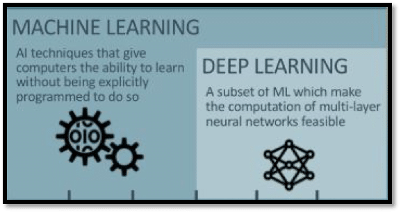
The formal definition of ML given by Arthur Samuel says “It provides computers with the capability to learn and take decisions without being explicitly programmed”.
Applications of ML includes Fraud Detection, Netflix Movie Recommendation etc. whereas Deep Learning can be defined as “Advanced Subset of Machine Learning” in which neural networks adapts and learns from vast amounts of data. It can be used to solve complex real-world problems such as self-driving cars, cancer detection. Let’s discuss each of them in detail.
What is Machine Learning?
As the name suggests, Machine Learning is all about the machine that learns. The question here is How do they learn? Machine Learning uses a mathematical function to construct a model based on training data which is then used to make predictions for the unknown data.
ML can be applied to a variety of domains such as finance, HR, Aerospace, pharmaceutical etc. There is a huge number of sophisticated algorithms available today to train the computers depending on the business problem. Some of them are Linear Regression, Logistic Regression, Random Forests, Support Vector Machines, neural networks. When there is a humongous amount of data available, the most intricate part is to select the correct algorithm to solve the problem. Each model has its own pros and cons and should be selected depending on the type of problem at hand and data available. We will not go into nitty gritty of each one of them.
Let’s try to build the predictive model for the HR department of XYZ company to understand the concept of Machine Learning in a better way. The aim of the model is to predict the number of employees who will leave the company in next five years based on factors such as Work satisfaction, Salary Increment, Number of hours spent in the office, promotion rate, last evaluation etc. The model also predicts the major cause due to which employees are leaving the company. In this way, the machine learning model will help the company to take the best measures to retain their employees in the next five years.
Neural Networks
One of the most important concepts of Machine Learning is Neural Networks. Let’s talk a bit about the Neural Network to go one step ahead towards the term “Deep Learning”. The idea of neural networks evolved from the dream to develop the algorithms that try to mimic the human brain. The simplest definition of a neural network is provided by Dr. Robert Hecht-Nielsen says a computing system made up of number of simple, highly interconnected processing elements, which process information by their dynamic state response to external inputs.
Why we need Neural Networks?
ML algorithms such as Linear Regression and Logistic Regression becomes convoluted while learning complex non-linear hypothesis. Above algorithms hold good when the number of features is less which is a rare case while solving real-world ML problems. Usually, the number of features in ML problems are more than 100 so we end up having the algorithm with an order of 5000 or more for a quadratic polynomial. It becomes computationally expensive. Moreover, the problem of overfitting arises because of which hypothesis presented by these algorithms couldn’t be generalized for new inputs. In such cases, these machine learning algorithms could be destructive.
Let’s understand the big picture of Neuron model:
Machine Learning Mode
Deep Learning Mode
Neuron Model:
The neuron model basically consists of 3 layers: an Input layer, Hidden Layer and Output Layer. Training data is provided to the input layer. Hidden layer is the computational unit which is called as “Sigmoid activationfunction”. Computation unit is nothing but the model which takes the input from the input layer and develops the hypothesis which is channeled down to the output layer. Aggregation of a large number of neuron models collectively known as Neural Networks.
Let’s refer to the model which predicts the number of employees who will leave the company in the next five years. Machine Learning algorithms such as Linear Regression, Logistic Regression holds good in this case because we have a limited number of features such as Work satisfaction, Salary increment, and limited training data available. But if we add the hundred more features such as department, Time spent in company, work accidents. Addition of these features will make the model nonlinear which can’t be solved by above-stated algorithms. This limitation can be overcome by the implementation of neural networks.
The complexity of the problem increases with a tremendous number of features and training data coming into picture due to which the efficiency of neural networks starts degrading. To improve the performance and capabilities of neural networks, the number of hidden layers in a neural network is increased. That’s where the Buzzword, “Deep Learning” comes into the picture.
Deep Learning Models:
Artificial Neural Networks are Machine Learning algorithms with one or two hidden layers whereas Deep Learning models consist of multiple hidden layers which help to improve the state of art technology to great extent. Addition of multiple hidden layers will make the network deep and is called Deep Learning.
Another major difference between Machine Learning and Deep Learning is Feature abstraction for a model. Domain expertise is critical in machine learning algorithm since a lot of preprocessing is required to clean the data and extracting the useful features which can be used to train the Machine Learning model. On the contrary, Deep Learning models learn in a more structured way to extract the features from raw data. As discussed in the above point, DL models consist of multiple hidden layers. Each hidden layer is used to identify one unique feature. DL models cut down the time consuming and arduous task of feature extraction.
There are a huge number of ML algorithms available which can be applied in a wide range of domains. Some of them are K means clustering, K nearest neighbors etc. The use of algorithms varies widely in ML depending on the application whereas, in the case of DL, the same piece of software can be trained for language translation as well as voice cloning. It all depends on the type of data that is fed to computers.
Let’s talk about real world example “Language Translators” to compare the efficiency of ML and DL models. Google launched the Chinese to English translator which used to translate the sentences phrase by phrase. This is far away from how humans translate. The efficiency of a model is around 78%. An upgraded version of language translators was launched recently which was based on Deep Learning model. This language translator model translates sentence by sentence rather than phrase by phrase which increased the efficiency of the model to 91%. DL models have also helped to increase the efficiency in areas of Image Recognition. The efficiency of ML based model for image recognition is 89% which increased up to 93% in the case of Deep Learning model.
The high efficiency comes at expense of stringent requirements:
Requirement of a huge amount of data to train the neural network with multiple layers.
Computationally expensive to train large scale neural networks.
It takes hours to train Deep Learning model since they process a large amount of data to parameterize the model.
Although the above requirements can be easily met with technological advancements, it is very important to choose the optimal model depending upon business problem and data available. Otherwise, DL models could be overkill for trivial application such as detection of spam email or movie recommendations.
Never thought that online trading could be so helpful because of so many scammers online until I met Miss Judith... Philpot who changed my life and that of my family. I invested $1000 and got $7,000 Within a week. she is an expert and also proven to be trustworthy and reliable. Contact her via: Whatsapp: +17327126738 Email:judithphilpot220@gmail.comread more
A very big thank you to you all sharing her good work as an expert in crypto and forex trade option. Thanks for... everything you have done for me, I trusted her and she delivered as promised. Investing $500 and got a profit of $5,500 in 7 working days, with her great skill in mining and trading in my wallet.
judith Philpot company line:... WhatsApp:+17327126738 Email:Judithphilpot220@gmail.comread more
Faculty knowledge is good but they didn't cover most of the topics which was mentioned in curriculum during online... session. Instead they provided recorded session for those.read more
Dimensionless is great place for you to begin exploring Data science under the guidance of experts. Both Himanshu and... Kushagra sir are excellent teachers as well as mentors,always available to help students and so are the HR and the faulty.Apart from the class timings as well, they have always made time to help and coach with any queries.I thank Dimensionless for helping me get a good starting point in Data science.read more
My experience with the data science course at Dimensionless has been extremely positive. The course was effectively... structured . The instructors were passionate and attentive to all students at every live sessions. I could balance the missed live sessions with recorded ones. I have greatly enjoyed the class and would highly recommend it to my friends and peers.
Special thanks to the entire team for all the personal attention they provide to query of each and every student.read more
It has been a great experience with Dimensionless . Especially from the support team , once you get enrolled , you... don't need to worry about anything , they keep updating each and everything. Teaching staffs are very supportive , even you don't know any thing you can ask without any hesitation and they are always ready to guide . Definitely it is a very good place to boost careerread more
The training experience has been really good! Specially the support after training!! HR team is really good. They keep... you posted on all the openings regularly since the time you join the course!! Overall a good experience!!read more
Dimensionless is the place where you can become a hero from zero in Data Science Field. I really would recommend to all... my fellow mates. The timings are proper, the teaching is awsome,the teachers are well my mentors now. All inclusive I would say that Kush Sir, Himanshu sir and Pranali Mam are the real backbones of Data Science Course who could teach you so well that even a person from non- Math background can learn it. The course material is the bonus of this course and also you will be getting the recordings of every session. I learnt a lot about data science and Now I find it easy because of these wonderful faculty who taught me. Also you will get the good placement assistance as well as resume bulding guidance from Venu Mam. I am glad that I joined dimensionless and also looking forward to start my journey in data science field. I want to thank Dimensionless because of their hard work and Presence it made it easy for me to restart my career. Thank you so much to all the Teachers in Dimensionless !read more
Dimensionless has great teaching staff they not only cover each and every topic but makes sure that every student gets... the topic crystal clear. They never hesitate to repeat same topic and if someone is still confused on it then special doubt clearing sessions are organised. HR is constantly busy sending us new openings in multiple companies from fresher to Experienced. I would really thank all the dimensionless team for showing such support and consistency in every thing.read more
I had great learning experience with Dimensionless. I am suggesting Dimensionless because of its great mentors... specially Kushagra and Himanshu. they don't move to next topic without clearing the concept.read more
My experience with Dimensionless has been very good. All the topics are very well taught and in-depth concepts are... covered. The best thing is that you can resolve your doubts quickly as its a live one on one teaching. The trainers are very friendly and make sure everyone's doubts are cleared. In fact, they have always happily helped me with my issues even though my course is completed.read more
I would highly recommend dimensionless as course design & coaches start from basics and provide you with a real-life... case study. Most important is efforts by all trainers to resolve every doubts and support helps make difficult topics easy..read more
Dimensionless is great platform to kick start your Data Science Studies. Even if you are not having programming skills... you will able to learn all the required skills in this class.All the faculties are well experienced which helped me alot. I would like to thanks Himanshu, Pranali , Kush for your great support. Thanks to Venu as well for sharing videos on timely basis...😊
I highly recommend dimensionless for data science training and I have also been completed my training in data science... with dimensionless. Dimensionless trainer have very good, highly skilled and excellent approach. I will convey all the best for their good work. Regards Avneetread more
After a thinking a lot finally I joined here in Dimensionless for DataScience course. The instructors are experienced &... friendly in nature. They listen patiently & care for each & every students's doubts & clarify those with day-to-day life examples. The course contents are good & the presentation skills are commendable. From a student's perspective they do not leave any concept untouched. The step by step approach of presenting is making a difficult concept easier. Both Himanshu & Kush are masters of presenting tough concepts as easy as possible. I would like to thank all instructors: Himanshu, Kush & Pranali.read more
When I start thinking about to learn Data Science, I was trying to find a course which can me a solid understanding of... Statistics and the Math behind ML algorithms. Then I have come across Dimensionless, I had a demo and went through all my Q&A, course curriculum and it has given me enough confidence to get started. I have been taught statistics by Kush and ML from Himanshu, I can confidently say the kind of stuff they deliver is In depth and with ease of understanding!read more
If you love playing with data & looking for a career change in Data science field ,then Dimensionless is the best... platform . It was a wonderful learning experience at dimensionless. The course contents are very well structured which covers from very basics to hardcore . Sessions are very interactive & every doubts were taken care of. Both the instructors Himanshu & kushagra are highly skilled, experienced,very patient & tries to explain the underlying concept in depth with n number of examples. Solving a number of case studies from different domains provides hands-on experience & will boost your confidence. Last but not the least HR staff (Venu) is very supportive & also helps in building your CV according to prior experience and industry requirements. I would love to be back here whenever i need any training in Data science further.read more
It was great learning experience with statistical machine learning using R and python. I had taken courses from... Coursera in past but attention to details on each concept along with hands on during live meeting no one can beat the dimensionless team.read more
I would say power packed content on Data Science through R and Python. If you aspire to indulge in these newer... technologies, you have come at right place. The faculties have real life industry experience, IIT grads, uses new technologies to give you classroom like experience. The whole team is highly motivated and they go extra mile to make your journey easier. I’m glad that I was introduced to this team one of my friends and I further highly recommend to all the aspiring Data Scientists.read more
It was an awesome experience while learning data science and machine learning concepts from dimensionless. The course... contents are very good and covers all the requirements for a data science course. Both the trainers Himanshu and Kushagra are excellent and pays personal attention to everyone in the session. thanks alot !!read more
Had a great experience with dimensionless.!! I attended the Data science with R course, and to my finding this... course is very well structured and covers all concepts and theories that form the base to step into a data science career. Infact better than most of the MOOCs. Excellent and dedicated faculties to guide you through the course and answer all your queries, and providing individual attention as much as possible.(which is really good). Also weekly assignments and its discussion helps a lot in understanding the concepts. Overall a great place to seek guidance and embark your journey towards data science.read more
Excellent study material and tutorials. The tutors knowledge of subjects are exceptional. The most effective part... of curriculum was impressive teaching style especially that of Himanshu. I would like to extend my thanks to Venu, who is very responsible in her jobread more
It was a very good experience learning Data Science with Dimensionless. The classes were very interactive and every... query/doubts of students were taken care of. Course structure had been framed in a very structured manner. Both the trainers possess in-depth knowledge of data science dimain with excellent teaching skills. The case studies given are from different domains so that we get all round exposure to use analytics in various fields. One of the best thing was other support(HR) staff available 24/7 to listen and help.I recommend data Science course from Dimensionless.read more
I was a part of 'Data Science using R' course. Overall experience was great and concepts of Machine Learning with R... were covered beautifully. The style of teaching of Himanshu and Kush was quite good and all topics were generally explained by giving some real world examples. The assignments and case studies were challenging and will give you exposure to the type of projects that Analytics companies actually work upon. Overall experience has been great and I would like to thank the entire Dimensionless team for helping me throughout this course. Best wishes for the future.read more
It was a great experience leaning data Science with Dimensionless .Online and interactive classes makes it easy to... learn inspite of busy schedule. Faculty were truly remarkable and support services to adhere queries and concerns were also very quick. Himanshu and Kush have tremendous knowledge of data science and have excellent teaching skills and are problem solving..Help in interviews preparations and Resume building...Overall a great learning platform. HR is excellent and very interactive. Everytime available over phone call, whatsapp, mails... Shares lots of job opportunities on the daily bases... guidance on resume building, interviews, jobs, companies!!!! They are just excellent!!!!! I would recommend everyone to learn Data science from Dimensionless only 😊read more
I am very glad to be part of Dimensionless .Their dedication, in-depth knowledge, teaching and the way they explain to... clarify doubts is tremendous . I recommend this to everyone who wish to build their career in Data Science
With whole heartedly I wish them for their success & future prospectsread more
Being a part of IT industry for nearly 10 years, I have come across many trainings, organized internally or externally,... but I never had the trainers like Dimensionless has provided. Their pure dedication and diligence really hard to find. The kind of knowledge they possess is imperative. Sometimes trainers do have knowledge but they lack in explaining them. Dimensionless Trainers can give you ‘N’ number of examples to explain each and every small topic, which shows their amazing teaching skills and In-Depth knowledge of the subject. Himanshu and Kush provides you the personal touch whenever you need. They always listen to your problems and try to resolve them devotionally.
I am glad to be a part of Dimensionless and will always come back whenever I need any specific training in Data Science. I recommend this to everyone who is looking for Data Science career as an alternative.
All the best guys, wish you all the success!!read more