If you are a working professional looking for your first Data Science stint or a student dreaming of building Jarvis, this blog will help you take your first baby step.
Python has literally 100s of libraries that make a Data Scientist’s life easier. It can be overwhelming for a beginner to think about learning all of these. This blog will introduce you to the 3 basic libraries popular among Data Scientists – Pandas, NumPy and RegEx.
Requirements:
- Jupyter Notebook
- Pandas, NumPy, RegEx libraries
- Download the Data from here – https://www.kaggle.com/c/titanic
- Some basic syntax knowledge of Python (lists, dictionaries, tuples,…)
Pandas
Unlike the obvious hunch, Pandas stands for ‘Panel Data’ and not a cute round animal. Widely used for handling data with multiple attributes, Pandas provides extremely handy commands to handle such data smoothly. Let’s move on to the coding exercises to get friendly with Pandas.
This section will cover the following:
- Loading datasets in Python
- Summarizing data
- Slicing data
- Treating missing values
Reading CSV files
Copy the file path. As you paste it, replace ‘\’ with ‘/’ The above command helps you to read a dataframe. Here, we have data in CSV format. You can also read xlsx, tsv, txt and several other file types. just type pd.read and press tab key. You will see a list of commands you can use to read files with various extensions.

Basic Pandas commands
df.head()
To view the first 5 rows of the data. Just to get a gist of how the data looks like. In case you want to view 3 or 6 or even 10 rows, use df.head(3) or df.head(6) or df.head(10). Take a second to view the dataframe.

df.shape()
The output is a tuple object with the first element equal to the number of rows (891) and the second element equal to the number of columns (12).

df.describe()
The output says what this command does. It provides summary statistics of variables (columns) with numeric entries. Hence, you won’t see any summary of columns like Name or Cabin. But, pandas still treats categorical variables like PClass as a continuous variable. We have to inform pandas to treat it the other way. This is done using ‘astyping’.

Slicing
Slicing here refers to selecting a piece of a dataframe. Say first 100 rows or the first 10 column. Pandas offer multiple simple ways to slice a dataframe. Below, we have slicing using column names and using dataframe.loc function.

Slicing with .loc using multiple columns

Similar to loc, we have ‘iloc’ which slices using only numbers to specify the row and the column ranges.

Instead of PassengerId, we have the column index (which is 0). Also notice that unlike ‘loc’,’iloc’ does not include the 29th entry. for x:y, iloc extends only till y-1.
Selecting a range of rows and columns:

To select something from the beginning, you needn’t write [0:final_point]. You can drop the 0,

Missing Value Imputation
Some entries of certain columns may be absent due to multiple reasons. Such values are called NA values. This function returns the count of missing values in each of our columns. Looks like we have 177 missing ages, 687 missing Cabin entries and 2 Embarked values.

There are multiple ways to impute NA values. A simple way is to replace them with mean, median or mode. Or even drop the data point. Let’s drop the two rows missing Embarked entry.
![]()
We fill NA values in Age with the mean of ages
![]()
Since 687 out of now 889 data points have missing Cabin entries, we drop the Cabin column itself.
![]()
NumPy
NumPy is a powerful package for scientific computing in Python. It is a Python library that provides a multidimensional array object, various derived objects (such as masked arrays and matrices), and an assortment of routines for fast operations on arrays, including mathematical, logical, shape manipulation, sorting, selecting, I/O, discrete Fourier transforms, basic linear algebra, basic statistical operations, random simulation and much more.
Let’s explore basic array creation in NumPy
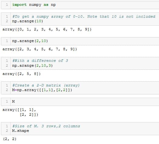
We can also create arrays with dimensions >=3

Maximum and Minimum Elements

The first element in the first row (0 index) is max along that row. Similarly the first element in the second row.

Changing axis to 0 reports index of the max element along a column.

Not specifying any axis returns the index of the max element in the array as if the array is flattened.

Output shows [1,1] indicating the element index of the minimum element in each row.

Similar to argmax
Sorting
Along row

Along column

Matrix Operations
We can perform almost any matrix operation in a couple of lines using NumPy. The following examples are self-evident.


RegEx
So far we have seen Python packages that help us handle numeric data. But what if the data is in the form of strings? RegEx is one such library that helps us handle such data. In this blog, we will introduce RegEx with some of its basic yet powerful functions.
A regular expression is a special text string for describing a search pattern. For example, we can define a special string to find all the uppercase characters in a text. Or we can define a special string that checks the presence of any punctuation in a text. You will gain more clarity once you start with the tutorial. It is highly advisable to keep this cheat sheet handy. This cheat sheet has all the building blocks you need to write a regular expression. We will try a few of these in this tutorial, but feel free to play around with the rest of them.

Above, we have imported the RegEx library and defined text which contains a string of characters.
Matching a string
re.match attempts a match with the beginning of a string. For example, here we try to locate any uppercase letters (+ denotes one or more) at the beginning of a string. r’[A-Z]+’ can be broken down as follow:
[A-Z]: Capture all the uppercase characters
+: Occurring once or more
As a result, the output is the string MY.

Searching a string
Unlike re.match, re.search does not limit itself to the beginning of the text. As soon as it finds a matching string in the text, it stops. In the example below, we match any uppercase letters (+ denotes one or more) at the beginning of a string. Take a look at the examples below

Finding all possible matches
re.findall as the name suggests, it returns a list of all possible non-overlapping matches in the string.
In the example below, r'[A-Z]’ looks for all uppercase letters.

Notice the difference in the output when we add a ‘+’ next to [A-Z]

Including ‘^’ implies that the match has to be made at the beginning of text:

‘.’ means any character. r’^[A-Z].’ says from the beginning, find an Uppercase letter. This can be followed by any character,

\d means a single digit. r’^[A-Z].’ says from the beginning, find an Uppercase letter. This can be followed by any digit (0-9). Since such a string does not exist in our text, we get an empty list.

\s means a whitespace. r’^[A-Z].’ says from the beginning, find an uppercase letter. This can be followed by any whitespace (denoted by \s). Since such a string does not exist in our text, we get an empty list.

‘\.’ avoids ‘.’ being treated as any character. ‘\.’ asks the findall function to skip any ‘.’ character seen

Substituting Strings
We can also substitute a string with another string using re.
Syntax – re.sub(“string to be replaced”,”string to be replaced with”,”input”)
