
In this article, we will be covering multiple linear regression model. We will also look at some important assumptions that should always be taken care of before making a linear regression model. We will also try to improve the performance of our regression model.
Multiple linear regression is a statistical technique that uses several explanatory variables to predict the outcome of a response variable. The goal of multiple linear regression is to model the relationship between the dependent and independent variables. We call it “multiple” because in this case, unlike simple linear regression, we have many independent variables trying to predict a dependent variable. For example, predicting cab price based on fuel price, vehicle cost and profits made by cab owners or predicting salary of an employee based on previous salary, qualifications, age etc.
Multiple linear regression models can be depicted by the equation

- y is a dependent variable which you are trying to predict. In linear regression, it is always a numerical variable and cannot be categorical
- x1, x2, and x3 are independent variables which are taken into the consideration to predict the dependent variable y
- a1, a2, a3 are coefficients which determine how a unit change in one variable will independently bring change in the final value you are trying to predict i.e a change in x3 by 1 unit will bring a change in our dependent variable y by an amount “a3” assuming a1 and a2 have remained constant
- a0 is also known as constant or the intercept value i.e. the value our predictor will output if there is no effect of any independent variables(x1, x2, x3) on our dependent variable(y)
Problem Statement: Predict cab price from my apartment to my office which has been off late fluctuating. Unlike my previous article on simple linear regression, cab price now not just depends upon the time I have been in the city but also other factors like fuel price, number of people living near my apartment, vehicle price in the city and lot other factors. We will try to build a model which can take all these factors into the consideration.
Let us start analyzing the data we have for this case. If you are new to regression and want to understand the basics, you may like to visit my previous article on the basics of regression.
Loading data set
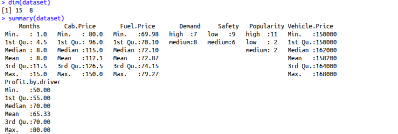
Load data set and study the structure of data set. “dim” function shows the dimension of the dataset. You can also see in the console that dim outputs result 15,8 meaning our data set has 15 rows and 8 columns. “summary” function, on the other hand, gives more detailed information about every column in the dataset. We should always try to understand the data first before jumping directly to the model building.
dataset <- read.csv("data.csv")
dim(dataset)
summary(dataset)
Handling categorical variables
We should always keep in mind that regression will take only continuous and discrete variables as input. In our case, 3 of our variables i.e. demand, safety, and popularity are categorical variables. These variables can not be used directly to build our regression model and hence we need to convert them to into a numeric one. We can do this by giving numeric levels to our categorical variables. We will replace low by a numeric -1, the medium by numeric 0 and high by numeric 1. We will repeat the same step for other categorical variables like safety and popularity.
#Converting demand variable into the factors
dataset$Demand = factor(dataset$Demand,
                       levels = c('low', 'medium', 'high'),
                       labels = c(-1, 0, 1))
#Converting safety variable into the factors
dataset$Safety = factor(dataset$Safety,
                        levels = c('low', 'medium', 'high'),
                        labels = c(-1, 0, 1))
#Converting popularity variable into factors
dataset$Popularity = factor(dataset$Popularity,
                        levels = c('low', 'medium', 'high'),
                        labels = c(-1, 0, 1))
Model Building
We will now directly build our multiple linear regression model. It is fairly simple to do and is done by using the lm function(in R). The first parameter is a formula which expects your dependent variable first followed by “~” and then all of the independent variables through which you want to predict your final dependent variable.
# Splitting the data set into the Training set and Test set

library(caTools)
set.seed(123)
split = sample.split(dataset$Cab.Price, SplitRatio = 0.8)
training_set = subset(dataset, split == TRUE)
test_set = subset(dataset, split == FALSE)
# Building multiple regression model with all the independent variables
regressor = lm(formula = training_set$Cab.Price ~ .,
               data = training_set)
Let us a take a break from model building here and understand the first few things which will help us to judge how good is the model which we have built
After building our multiple regression model let us move onto a very crucial step before making any predictions using out model. There are some assumptions that need to be taken care of before implementing a regression model. All of these assumptions must hold true before you start building your linear regression model.

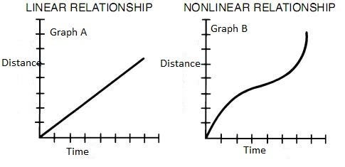
- Assumption 1: Relationship between your independent and dependent variables should always be linear i.e. you can depict a relationship between two variables with help of a straight line. Let us check whether this assumption holds true or not for our case.
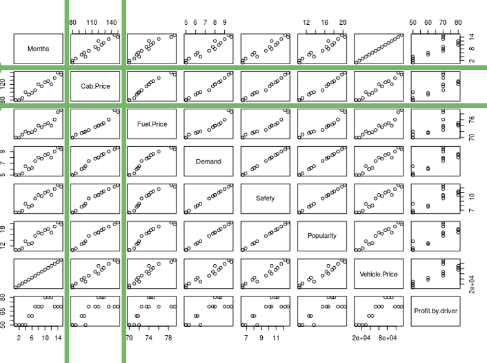
By looking at the second row and second column, we can say that our independent variables posses linear relationship(observe how scatterplots are more or less giving a shape of a line) with our dependent variable(cab price in our case)
- Assumption 2: Mean of residuals should be zero or close to 0 as much as possible. It is done to check whether our line is actually the line of “best fit”.

We want the arithmetic sum of these residuals to be as much equal to zero as possible as that will make sure that our predicted cab price is as close to actual cab price as possible. In our case, mean of the residuals is also very close to 0 hence the second assumption also holds true.
> mean(regressor$residuals)
[1] 6.245005e-17
- Assumption 3: There should be homoscedasticity or equal variance in our regression model. This assumption means that the variance around the regression line is the same for all values of the predictor variable (X). The sample plot below shows a violation of this assumption. For the lower values on the X-axis, the points are all very near the regression line. For the higher values on the X-axis, there is much more variability around the regression line.
To check homoscedasticity, we make a plot of residual values on the y-axis and the predicted values on the x-axis. If we see a bell curve, then we can say that there is no homoscedasticity. It means that the variability of a variable is unequal across the range of values of a second variable that predicts it.
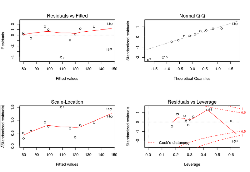
par(mfrow=c(2,2))  # set 2 rows and 2 column plot layout
plot(regressor)
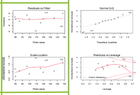
From the first plot (top-left), as the fitted values along x increase, the residuals remain more or less constant. This pattern is indicated by the red line, which should be approximately flat if the disturbances are homoscedastic. The plot on the bottom left also checks this and is more convenient as the disturbance term in the Y-axis is standardized. The points appear random and the line looks pretty flat(top-left graph), with no increasing or decreasing trend. So, the condition of homoscedasticity can be accepted.
- Assumption 4: All the dependent variables and residuals should be uncorrelated.
cor.test(training_set$Months, regressor$residuals)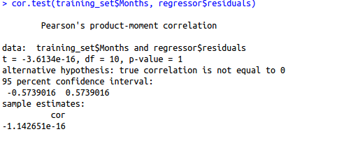
Here, our null hypothesis is that there is no relationship between our independent variable Months and the residuals while the alternate hypothesis will be that there is a relationship between months and residuals. Since the p-value is very high, we can not reject the null hypothesis and hence our assumption holds true for this variable for this model. We need to repeat this step for other independent variables also.
- Assumption 5: Number of observations should be greater than the number of independent variables. We can check this by directly looking at our data set only.
- Assumption 6: There should be no perfect multicollinearity in your model. Multicollinearity generally occurs when there are high correlations between two or more independent variables. In other words, one independent variable can be used to predict the other. This creates redundant information, skewing the results in a regression model. We can check multicollinearity using VIF(variance inflation factor). Higher the VIF for an independent variable, more is the chance that variable is already explained by other independent variables.
- Assumption 7: Residuals should be normally distributed. This can be checked by visualizing Q-Q Normal plot. If points lie exactly on the line, it is perfectly normal distribution. However, some deviation is to be expected, particularly near the ends (note the upper right), but the deviations should be small, even lesser than they are here.
Checking assumptions automatically
We can use the gvlma library to evaluate the basic assumptions of linear regression for us automatically.
library(gvlma)
regressor = lm(formula = training_set$Cab.Price ~ training_set$Demand + training_set$Fuel.Price +training_set$Vehicle.Price+training_set$Profit.by.driver,
               data = training_set)
gvlma(regressor)
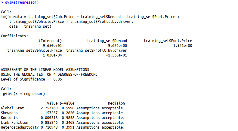

Are you finding it difficult to understand the output of the gvlma() function? Let us understand this output in detail.
1. Global Stat: It measures the linear relationship between our independent variables and the dependent variable which we are trying to predict. The null hypothesis is that there is a linear relationship between our independent and dependent variables. Since our p-value >0.05, we can easily accept our null hypothesis and conclude that there is indeed a linear relationship between our independent and dependent variables.
2. Skewness: Data can be “skewed”, meaning it tends to have a long tail on one side or the other
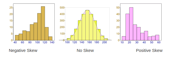
- Negative Skew: The long tail is on the “negative” (left) side of the peak. Generally, the mean < median < mode in this case.
- No Skew: There is no observed tail on any side of the peak. It is always symmetrical. Mean, median and mode are at the center of the peak i.e. mean = m0edian = mode
- Positive Skew: The long tail is on the “positive” (right) side of the peak. Generally, mode < median < mean in this case.
We want our data to be normally distributed. The second assumption looks for skewness in our data. The null hypothesis states that our data is normally distributed. In our case, since the p-value for this is >0.05, we can safely conclude that our null hypothesis holds hence our data is normally distributed.
3. Kurtosis: The kurtosis parameter is a measure of the combined weight of the tails relative to the rest of the distribution. It measures the tail-heaviness of the distribution. Although not correct, you can indirectly relate kurtosis to shape of the peak of normal distribution i.e. whether your normal distribution as a sharp peak or a shallow peak.
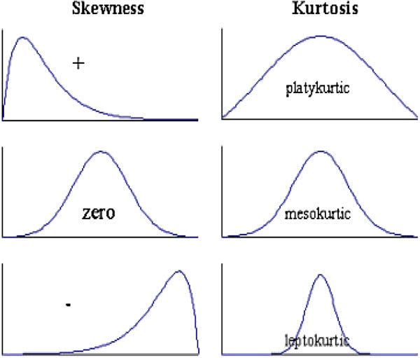
- Mesokurtic: This is generally the ideal scenario where your data has a normal distribution.
- Platykurtic(negative kurtosis score): A flatter peak is observed in this case because there are fewer data in your dataset which resides in the tail of the distribution i.e. tails are thinner as compared to the normal distribution. It has a shallower peak than normal which means that this distribution has thicker tails and that there are fewer chances of extreme outcomes compared to a normal distribution.
- Leptokurtic(positive kurtosis score): A sharper peak is observed as compared to normal distribution because there is more data in your dataset which resides in the tail of the distribution as compared to the normal distribution. It has a lesser peak than normal which means that this distribution has fatter tails and that there are more chances of extreme outcomes compared to a normal distribution.
We want our data to be normally distributed. The third assumption looks for the amount of data present in the tail of the distribution. The null hypothesis states that our data is normally distributed. In our case, since the p-value for this is >0.05, we can safely conclude that our null hypothesis holds hence our data is normally distributed.
4. Link function: It tells us whether our dependent function is numeric or categorical. As I have already mentioned before, for linear regression your dependent variable should be numeric and not categorical. The null hypothesis states that our dependent variable is numeric. Since the p-value for this case is again > 0.05, our null hypothesis holds true hence we can conclude that our dependent variable is numeric.
5. Heteroscedasticity: Is the variance of your model residuals constant across the range of X (assumption of homoskedasticity(discussed above in assumptions))? Rejection of the null (p < .05) indicates that your residuals are heteroscedastic, and thus non-constant across the range of X. Your model is better/worse at predicting for certain ranges of your X scales.
As we can observe, the gvlma function has automatically tested our model for 5 basic assumptions in linear regression and woohoo, our model has passed all the basic assumptions of linear regression and hence is a qualified model to predict results and understand the influence of independent variables (predictor variables) on your dependent variable
Understanding R squared and Adjusted R Squared
R-squared is a statistical measure of how close the data are to the fitted regression line. It is also known as the coefficient of determination, or the coefficient of multiple determination for multiple regression. It can also be defined as the percentage of the response variable variation that is explained by a linear model.
R-squared = Explained variation / Total variation
R-squared is always between 0 and 100%:
0% indicates that the model explains none of the variability of the response data around its mean.
100% indicates that the model explains all the variability of the response data around its mean.
In general, the higher the R-squared, the better the model fits your data.
But R-squared cannot determine whether the coefficient estimates and predictions are biased, which is why we must assess the residual plots. However, R-squared has additional problems that the adjusted R-squared and predicted R-squared is designed to address.

Problem 1: Whenever we add a new independent variable(predictor) to our model, R-squared value always increases. It will not depend upon whether the new predictor variable holds much significance in the prediction or not. We may get lured to increase our R squared value as much possible by adding new predictors, but we may not realize that we end up adding a lot of complexity to our model which will make it difficult to interpret.
Problem 2: If a model has too many predictors and higher order polynomials, it begins to model the random noise in the data. This condition is known as over-fitting and it produces misleadingly high R-squared values and a lessened ability to make predictions.
How adjusted R squared comes to our rescue
We will now have a look at how adjusted r squared deals with the shortcomings of r squared. To begin with, I will say that adjusted r squared modified version of R-squared that has been adjusted for the number of predictors in the model. The adjusted R-squared increases only if the new term improves the model more than would be expected by chance. It decreases when a predictor improves the model by less than expected by chance. The adjusted R-squared can be negative, but it’s usually not. It is always lower than the R-squared.
Let us understand adjusted R squared in more detail by going through its mathematical formula.
where n = number of points in our data set
k = number of independent variables(predictors) used to develop the model
From the formula, we can observe that, if we keep on adding too much of non-significant predictors then k will tend to increase while R squared won’t increase so much. Hence n-k-1 will decrease and the numerator will be almost the same as before. So then entire fraction will increase(since denominator has decreased with increased k). This will result in a bigger value being subtracted from 1 and we end up with a smaller adjusted r squared value. Hence this way, adjusted R squared compensates by penalizing us for those extra variables which do not hold much significance in predicting our target variable.
Let’s get back to the model we built and look at whether all the assumptions hold true for it or not and try to build a better model
library(gvlma)
regressor = lm(formula = training_set$Cab.Price ~ training_set$Demand + training_set$Fuel.Price +training_set$Vehicle.Price+training_set$Profit.by.driver,
               data = training_set)
gvlma(regressor)
summary(regressor)
Oops! It seems like there is an error while testing our model for assumptions of linear regression.

This error means your design matrix is not invertible and therefore can’t be used to develop a regression model. This results from linearly dependent columns, i.e. strongly correlated variables. Examine the pairwise covariance (or correlation) of your variables to investigate if there are many variables that can potentially be removed.
Let us have a look at detailed summary if we can find any anomalies there.
summary(regressor)
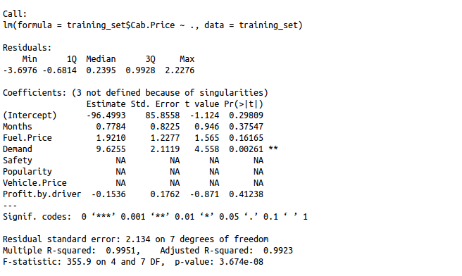
Seeing so many NA`s may indicate the features where exactly the problem lies. Let us check which columns are responsible for creating multicollinearity in our data set.
cor.test(training_set$Safety,training_set$Popularity)
cor.test(training_set$Popularity, training_set$Months)
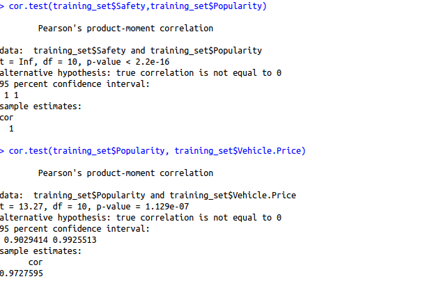
Since the p-value is quite close to 0 in both cases, we have to reject our null hypothesis ( There is no relationship between two features).On further investigation, it was found that demand also showed high collinearity with safety parameter. Hence demand safety, popularity and vehicle price can be deduced from each other. So out of these 3, we will take only 1 variable say demand (higher significance as shown by summary function) in this case.
regressor = lm(formula = Cab.Price ~ Months+Fuel.Price+Demand+Profit.by.driver, data = training_set)
gvlma(regressor)
summary(regressor)
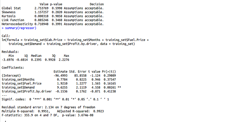
All assumptions are met but the summary method says that demand is the only significant variable in this case. Let us make our model a little less complex but removing some of the more variables. We will pick on the variables having higher p-values.
R squared: 0.9951
Adjusted R squared: 99.23
Removing “profit by driver” variable
regressor = lm(formula = training_set$Cab.Price ~ Months+Fuel.Price+Demand,
               data = training_set)
gvlma(regressor)
summary(regressor)
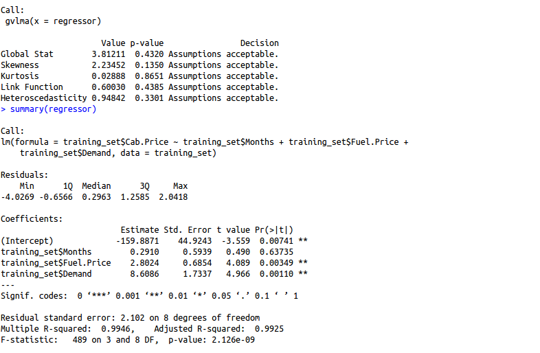
R squared: 0.9946
Adjusted R squared: 99.25
Observation: Removing profit by driver variable increased our adjusted R squared indicating that this feature was not much significant.
All assumptions met.
Removing the “Months” variable by the same logic as it is non-significant …
regressor = lm(formula = training_set$Cab.Price ~ Fuel.Price+Demand,
               data = training_set)
gvlma(regressor)
summary(regressor)
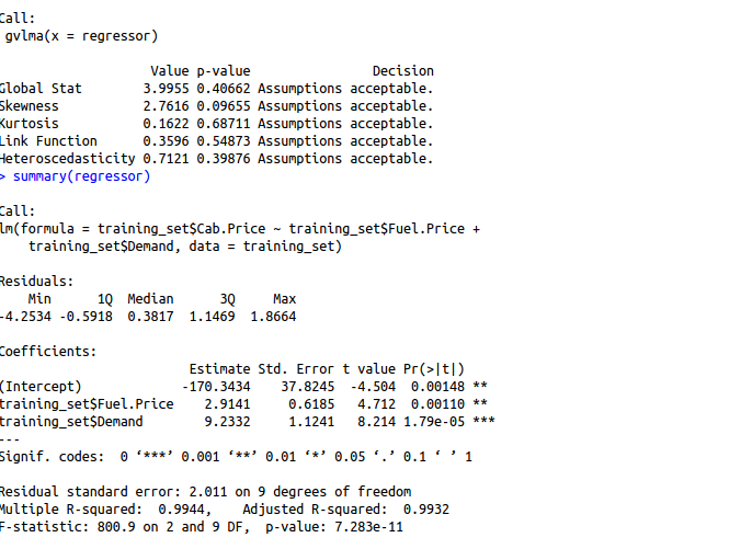
R squared: 0.9944
Adjusted R squared: 0.9932
Observation: Removing “months” variable increased our adjusted R squared indicating that this feature was not much significant either.
Finally, we have both significant variables with us and if you look closely we have highest Adjusted R squared with the model based out of two features (0.9932) as compared to the model with all the features (0.9922).
Finally, in this article, we were able to build a multiple regression model and were able to understand the maths behind. The aim was to not just build a model but to build one keeping in mind the assumptions and complexity of the model. Stay tuned for more articles on machine learning!