9923170071 / 8108094992 info@dimensionless.in
Top 10 Machine Learning Algorithms

Top 10 Machine Learning Algorithms

Introduction

Machine learning paradigm is ruled by a simple theorem known as “No Free Lunch” theorem. According to this, there is no algorithm in ML which will work best for all the problems. To state, one can not conclude that SVM is a better algorithm than decision trees or linear regression. Selection of an algorithm is dependent on the problem at hand and other factors like the size and structure of the dataset. Hence, one should try different algorithms to find a better fit for their use case

In this blog, we are going to look into the top machine learning algorithms. You should know and implement the following algorithms to find out the best one for your use case


Top 10 Best Machine Learning Algorithms


1. Linear Regression

Regression is a method used to predict numerical numbers. Regression is a statistical measure which tries to determine the power of the relation between the label-related characteristics of a single variable and other factors called autonomous (periodic attributes) variable. Regression is a statistical measure. Just as the classification is used for categorical label prediction, regression is used for ongoing value prediction. For example, we might like to anticipate the salary or potential sales of a new product based on the prices of graduates with 5-year work experience. Regression is often used to determine how the cost of an item is affected by specific variables such as product cost, interest rates, specific industries or sectors.

The linear regression tries by a linear equation to model the connection between a scalar variable and one or more explaining factors. For instance, using a linear regression model, one might want to connect the weights of people to their heights

The driver calculates a linear pattern of regression. It utilizes the model selection criterion Akaike. A test of the comparative value of fitness to statistics is the Akaike information criterion. It is based on the notion of entropy, which actually provides a comparative metric of data wasted when a specified template is used to portray the truth. The compromise between bias and variance in model building or between the precision and complexity of the model can be described.


2. Logistic Regression

Logistic regression is a classification system that predicts the categorical results variable that may take one of the restricted sets of category scores using entry factors. A binomial logistical regression is restricted to 2 binary outputs and more than 2 classes can be achieved through a multinomial logistic regression. For example, classifying binary conditions as’ safe’/’don’t-healthy’ or’ bike’ /’ vehicle’ /’ truck’ is logistic regression. Logistic regression is used to create an information category forecast for weighted entry scores by the logistic sigmoid function.
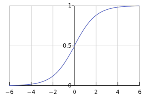
logistic regression graph


The probability of a dependent variable based on separate factors is estimated by a logistic regression model. The variable depends on the yield that we want to forecast, whereas the indigenous variables or explaining variables may affect the performance. Multiple regression means an assessment of regression with two or more independent variables. On the other side, multivariable regression relates to an assessment of regression with two or more dependent factors.


3. Linear Discriminant Analysis

Logistic regression is traditionally a two-class classification problem algorithm. If you have more than two classes, the Linear Discriminant Analysis algorithm is the favorite technique of linear classification. It contains statistical information characteristics, which are calculated for each category.

For a single input variable this includes:

  1. The mean value for each class.
  2. The variance calculated across all classes.
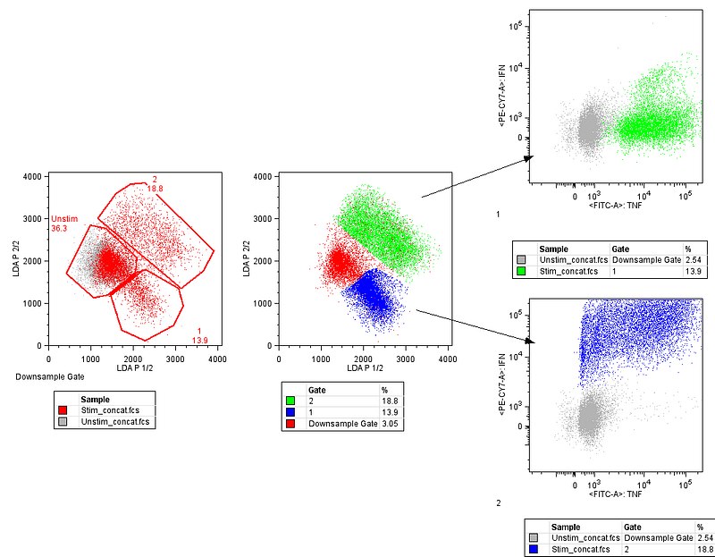
  3.  
Linear Discriminant Analysis algorithm


The predictions are calculated by determining a discriminating value for each class and by predicting the highest value for each class. The method implies that the information is distributed Gaussian (bell curve) so that outliers are removed from your information in advance. It is an easy and strong way to classify predictive problem modeling.


4. Classification and Regression Trees

Prediction Trees are used to forecast answer or YY class of X1, X2,…, XnX1,X2,… ,Xn entry. If the constant reaction is called a regression tree, it is called a ranking tree, if it is categorical. We inspect the significance of one entry XiXi at any point of the tree and proceed to the left or to the correct subbranch, based on the (binary) response. If we hit a tree, we will discover the forecast (generally the leaves as the most popular value of the accessible courses is a straightforward statistical figure of the dataset).
In contrast to global model linear or polynomial regression (a predictive formula should be contained in the whole data space), trees attempt to split the data space in a sufficiently small part, where a simply different model can be applied on each side. For each xx information, the non-leaf portion of the tree is simply the process to determine what model we use for the classification of each information (i.e. which leaf).
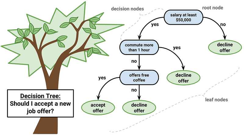
 

Regression Trees


5. Naive Bayes

A Naive Bayes classification is a supervised algorithm for machinery-learning which utilizes the theorem of Bayes, which implies statistical independence of its characteristics. The theorem depends on the naive premise that input factors are autonomous from each other, that is, that when an extra variable is provided there is no way to understand anything about other factors. It has demonstrated to be a classifier with excellent outcomes regardless of this hypothesis.
The Bavarian Theorem, relying on a conditional probability, or in easy words, is used for the Naive Bayes classifications as a probability of a case (A) occurring considering that another incident (B) has already occurred. In essence, the theorem enables an update of the hypothesis every moment fresh proof is presented.

The equation below expresses Bayes’ Theorem in the language of probability:

Bayes’ Theorem


Let’s explain what each of these terms means.

  • “P” is the symbol to denote probability.
  • P(A | B) = The probability of event A (hypothesis) occurring given that B (evidence) has occurred.
  • P(B | A) = The probability of the event B (evidence) occurring given that A (hypothesis) has occurred.
  • P(A) = The probability of event B (hypothesis) occurring.
  • P(B) = The probability of event A (evidence) occurring.


6. K-Nearest Neighbors

The KNN is a simple machine study algorithm which classifies an entry using its closest neighbours.
The input of information points of particular males and women’s height and weight as shown below should be provided, for instance, by a k-NN algorithm. K-NN can peer into the closest k neighbour (personal) and determine if the entry gender is masculine in order to determine the gender of an unidentified object (green point). This technique is extremely easy and logical, with a strong achievement level for labelling unidentified input.


 K-Nearest Neighbors


k-NN is used in a range of machine learning tasks; k-NN, for example, can help in computer vision in hand-written letters and the algorithm is used to identify genes that are contributing to a specific characteristic of the gene expression analysis. Overall, neighbours close to each other offer a mixture of ease and efficiency that makes it an appealing algorithm for many teaching machines.7. Learning Vector Quantization


8. Bagging and Random Forest

A Random Forest is a group of easy tree predictors, each of which is capable of generating an answer when it has a number of predictor values. This reaction requires the form of a class affiliation for classification issues, which combines or classifies a number of indigenous predictor scores with one of the classifications in the dependent variable. Otherwise, the tree reaction is an assessment of the dependent variable considering the predictors for regression difficulties. Breiman has created the Random Forest algorithm.
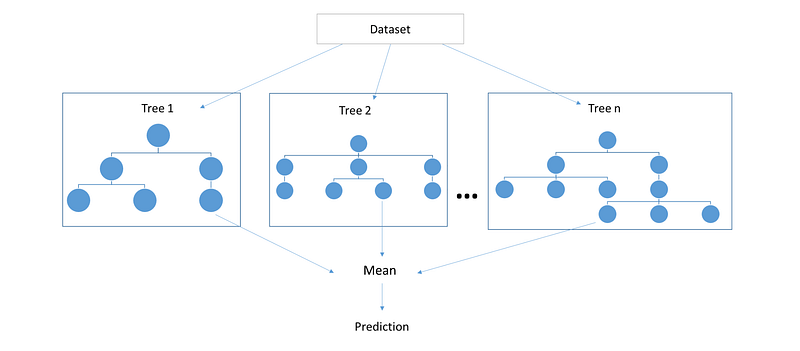
Image result for random forest


An arbitrary amount of plain trees are a random forest used to determine the ultimate result. The ensemble of easy trees votes for the most common category for classification issues. Their answers are averaged to get an assessment of the dependent variable for regression problems. With tree assemblies, the forecast precision (i.e. greater capacity to detect fresh information instances) can improve considerably.


9. SVM

The support vector machine(SVM) is a supervised, classifying, and regressing machine learning algorithm. In classification issues, SVMs are more common, and as such, we shall be focusing on that article.SVMs are based on the idea of finding a hyperplane that best divides a dataset into two classes, as shown in the image below.
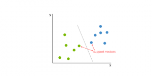
SVM graph


You can think of a hyperplane as a line that linearly separates and classifies a set of data.

The more our information points are intuitively located from the hyperplane, the more assured that they have been categorized properly. We would, therefore, like to see as far as feasible from our information spots on the right hand of the hyperplane.

So when new test data are added, the class we assign to it will be determined on any side of the hyperplane.

The distance from the hyperplane to the nearest point is called the margin. The aim is to select a hyperplane with as much margin as feasible between the hyperplane and any point in the practice set to give fresh information a higher opportunity to be properly categorized.
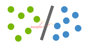
hyperplane


But the data is rarely ever as clean as our simple example above. A dataset will often look more like the jumbled balls below which represent a linearly non-separable dataset.

jumped balls dataset


It is essential to switch from a 2D perspective to a 3D perspective to classify a dataset like the one above. Another streamlined instance makes it easier to explain this. Imagine our two balls stood on a board and this booklet is raised abruptly, throwing the balls into the air. You use the cover to distinguish them when the buttons are up in the air. This “raising” of the balls reflects a greater identification of the information. This is known as kernelling.
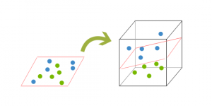
hyperlane

Our hyperplanes can be no longer a row because we are in three dimensions. It should be a flight now, as shown in the above instance. The concept is to map the information into greater and lower sizes until a hyperplane can be created to separate the information.


10. Boosting and AdaBoost

Boosting is an ensemble technology which tries to build a powerful classification of a set of weak classifiers. This is done using a training data model and then a second model has created that attempts the errors of the first model to be corrected. Until the training set is perfectly predicted or a maximum number of models are added, models are added.

AdaBoost was the first truly effective binary classification boosting algorithm. It is the best point of start for improvement. Most of them are stochastic gradient boosters, based on AdaBoost modern boosting techniques.
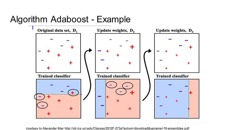
AdaBoost modern boosting techniques.


With brief choice trees, AdaBoost is used. After the creation of the first tree, each exercise instance uses the performance of the tree to weigh how much attention should be given to the next tree to be built. Data that are difficult to forecast will be provided more weight, while cases that are easily predictable will be less important. Sequentially, models are produced one by one to update each of the weights on the teaching sessions which impact on the study of the next tree. After all, trees have been produced, fresh information are predicted and how precise it was on the training data weighs the efficiency of each tree.

Since the algorithm is so careful about correcting errors, it is essential that smooth information is deleted with outliers.


Summary

In the end, every beginner in data science has one basic starting questions that which algorithm is best for all the cases. The response to the issue is not straightforward and depends on many factors like information magnitude, quality and type of information; time required for computation; the importance of the assignment; and purpose of information

Even an experienced data scientist cannot say which algorithm works best before distinct algorithms are tested. While many other machine learning algorithms exist, they are the most common. This is a nice starting point to understand if you are a beginner for machine learning.

Follow this link, if you are looking to learn data science online!

You can follow this link for our Big Data course!

Additionally, if you are having an interest in learning Data Science, click here to start the Online Data Science Course

Furthermore, if you want to read more about data science, read our Data Science Blogs

How to Make Machine Learning Models for Beginners

How to Make Machine Learning Models for Beginners

Introduction

Data science is one of the hottest topics in the 21st century because we are generating data at a rate which is much higher than what we can actually process. A lot of business and tech firms are now leveraging key benefits by harnessing the benefits of data science. Due to this, data science right now is really booming.

In this blog, we will deep dive into the world of machine learning. We will walk you through machine learning basics and have a look at the process of building an ML model. We will also build a random forest model in python to ease out the understanding process.


What is Machine Learning?

Machine Learning is the science of getting computers to learn and act like humans do, and improve their learning over time in an autonomous fashion, by feeding them data and information in the form of observations and real-world interactions.

There are many different types of machine learning algorithms, with hundreds published each day, and they’re typically grouped by either learning style (i.e. supervised learning, unsupervised learning, semi-supervised learning) or by similarity in form or function (i.e. classification, regression, decision tree, clustering, deep learning, etc.). Regardless of learning style or function, all combinations of machine learning algorithms consist of the following:

  • Representation (a set of classifiers or the language that a computer understands)
  • Evaluation (aka objective/scoring function)
  • Optimization (search method; often the highest-scoring classifier, for example; there are both off-the-shelf and custom optimization methods used)


Steps for Building ML Model

Here is a step-by-step example of how a hospital might use machine learning to improve both patient outcomes and ROI:

1. Define Project Objectives

The first step of the life cycle is to identify an opportunity to tangibly improve operations, increase customer satisfaction, or otherwise create value. In the medical industry, discharged patients sometimes develop conditions that necessitate their return to the hospital. In addition to being dangerous and troublesome for the patient, these readmissions mean the hospital will spend additional time and resources on treating patients for the second time.

2. Acquire and Explore Data

The next step is to collect and prepare all of the relevant data for use in machine learning. This means consulting medical domain experts to determine what data might be relevant in predicting readmission rates, gathering that data from historical patient records, and getting it into a format suitable for analysis, most likely into a flat file format such as a .csv.

3. Model Data

In order to gain insights from your data with machine learning, you have to determine your target variable, the factor of which you are trying to gain a deeper understanding. In this case, the hospital will choose “readmitted,” which is included as a feature in its historical dataset during data collection. Then, they will run machine learning algorithms on the dataset that build models that learn by example from the historical data. Finally, the hospital runs the trained models on data the model hasn’t been trained on to forecast whether new patients are likely to be readmitted, allowing it to make better patient care decisions.

4. Interpret and Communicate

One of the most difficult tasks of machine learning projects is explaining a model’s outcomes to those without any data science background, particularly in highly regulated industries such as healthcare. Traditionally, machine learning has been thought of as a “black box” because of how difficult it is to interpret insights and communicate their value to stakeholders and regulatory bodies alike. The more interpretable your model, the easier it will be to meet regulatory requirements and communicate its value to management and other key stakeholders.

5. Implement, Document, and Maintain

The final step is to implement, document, and maintain the data science project so the hospital can continue to leverage and improve upon its models. Model deployment often poses a problem because of the coding and data science experience it requires, and the time-to-implementation from the beginning of the cycle using traditional data science methods is prohibitively long.


Problem Statement

A certain car manufacturing company X is looking to target its customers for their particular car model. Customers are identified by their age, salary, and Gender. The organisation wants to identify or predict which customers will affect the sales of their new car and actually purchase it.

We have a purchased column here which holds two values i.e 0 and 1. 0 indicates that the car has not been purchased by a certain individual. 1 indicates the sale of the car.


Code Implementation

Importing the Required Libraries

You need to import all the required libraries first which will ease the model building parts for us. We are using keras to build our random forest model. We are using the matplotlib library to plot the charts and graphs and visualise results. In the end, we are also importing functions from the sklearn module which can help us in splitting our data into training and testing parts

# Importing the libraries
import numpy as np
import matplotlib.pyplot as plt
import pandas as pd
from sklearn.model_selection import train_test_split
from sklearn.ensemble import RandomForestClassifier


Loading the Dataset

In this step, you need to load your dataset in the memory. After that, we separate out the dependent and the independent variables for the training of our classifier. In most of the cases, you need to separate the dependent and he the independent variables

# Importing the dataset
dataset = pd.read_csv('Social_Network_Ads.csv')
X = dataset.iloc[:, [2, 3]].values
y = dataset.iloc[:, 4].values


Splitting the Dataset to Form Training and Test Data

In all the cases, you need to make some partitions in your data. A major chunk of your data acts as a training set and a smaller chunk acts as a test set. There are no clearly defined criteria on the proportion of the training and the test set. But most people follow 70–30 or 75–25 rule where a larger chunk is your training set. We train the data on the training set and test it on the test set. This process is known as validation. The prime idea behind this purpose is that one needs to gauge the performance of the model on the data which model has never seen before. In the real-world scenarios, the model will be predicting values on the unseen data. Furthermore, techniques like validation help us in avoiding overfitting or underfitting the model. 

Overfitting refers to the case when our model has learnt all about the specific data on which it trained. It will work well on the training data but will have poor accuracy for any unseen data point. Overfitting is like your model is very specific to the data it has and has no generality. Similarly, underfitting is the case where your model is very general and is not able to predict well for your specific use-case. To achieve the best model accuracy, you need to strike a perfect balance between overfitting and under-fitting.

# Splitting the dataset into the Training set and Test set
from sklearn.model_selection import train_test_split
X_train, X_test, y_train, y_test = train_test_split(X, y, test_size = 0.25, random_state = 0)


Standardising the Dataset Values

from sklearn.preprocessing import StandardScaler
sc = StandardScaler()
X_train = sc.fit_transform(X_train)
X_test = sc.transform(X_test)


Fitting a Random Forest Classifier

In this case, we are fitting our model with the training data. We are using the random forest model exposed by the sklearn package in python. Ultimately, we pass the dependent and independent features separately through which our model makes an internal mapping between them using mathematical coefficients.

# Fitting Random Forest Classification to the Training set
from sklearn.ensemble import RandomForestClassifier
classifier = RandomForestClassifier(n_estimators = 10, criterion = 'entropy', random_state = 0)
classifier.fit(X_train, y_train)


Predicting Results from the Classifier

In this part, we are passing unseen values to our model on which it is making predictions. We use a confusion matrix to derive metrics like accuracy, precision, and recall for our model. These metrics help us to understand the performance of the model.

# Predicting the Test set results
y_pred = classifier.predict(X_test)

# Making the Confusion Matrix
from sklearn.metrics import confusion_matrix
cm = confusion_matrix(y_test, y_pred)


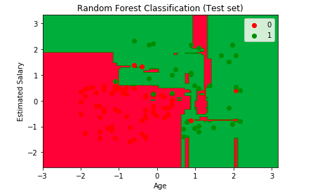
Visualising the Predictions

Additionally, we have made an attempt to visualise the predictions of our model using the below code.

# Visualising the Test set results
from matplotlib.colors import ListedColormap
X_set, y_set = X_test, y_test
X1, X2 = np.meshgrid(np.arange(start = X_set[:, 0].min() - 1, stop = X_set[:, 0].max() + 1, step = 0.01),
                     np.arange(start = X_set[:, 1].min() - 1, stop = X_set[:, 1].max() + 1, step = 0.01))
plt.contourf(X1, X2, classifier.predict(np.array([X1.ravel(), X2.ravel()]).T).reshape(X1.shape),
             alpha = 0.75, cmap = ListedColormap(('red', 'green')))
plt.xlim(X1.min(), X1.max())
plt.ylim(X2.min(), X2.max())
for i, j in enumerate(np.unique(y_set)):
    plt.scatter(X_set[y_set == j, 0], X_set[y_set == j, 1],
                c = ListedColormap(('red', 'green'))(i), label = j)
plt.title('Random Forest Classification (Test set)')
plt.xlabel('Age')
plt.ylabel('Estimated Salary')
plt.legend()
plt.show()


Summary

Hence, in this Machine Learning Tutorial, we studied the basics of ML. Earlier machine learning was the theory that computers can learn without being programmed to perform specific tasks. But now, the researchers interested in artificial intelligence wanted to see if computers could learn from data. They learn from previous computations to produce reliable decisions and results. It’s a science that’s not new — but one that’s gaining fresh momentum.

Follow this link, if you are looking to learn more about data science online!

You can follow this link for our Big Data course!

Additionally, if you are having an interest in learning Data Science, click here to start Best Online Data Science Courses 

Furthermore, if you want to read more about data science, you can read our blogs here

A Personal Digital Assets Manager – Blockchain Applications of Data Science Part 1

How to Write a Spark Application in Scala

Difference Between A Data Scientist and Statistician


Introduction to Random forest


Introduction

Random forest is one of those algorithms which comes to the mind of every data scientist to apply on a given problem. It has been around for a long time and has successfully been used for such a wide number of tasks that it has become common to think of it as a basic need. It is a versatile algorithm and can be used for both regression and classification.
This post aims at giving an informal introduction of Random Forest and its implementation in R.


Table of contents

  1. What is a Decision Tree?
  2. What is Random Forest?
  3. Random forest in R.
  4. Pros and Cons?
  5. Applications

What is a Decision Tree?

Best Essay Writing Service: Reddit Users Testimonials

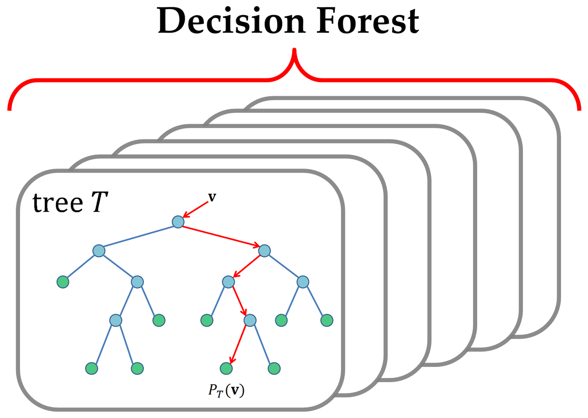
Decision tree is a simple, deterministic data structure for modelling decision rules for a specific classification problem. At each node, one feature is selected to make separating decision. We can stop splitting once the leaf node has optimally less data points. Such leaf node then gives us insight into the final result (Probabilities for different classes in case of classfication).
Refer the figure below for a clearer understanding:

decision_tree

How does it split?

The most decisive factor for the efficiency of a decision tree is the efficiency of its splitting process. We split at each node in such a way that the resulting purity is maximum. Well, purity just refers to how well we can segregate the classes and increase our knowledge by the split performed. An image is worth a thousand words. Have a look at the image below for some intuition:

gini

Two popular methods for splitting are:

  1. Gini Impurity
  2. Information Gain

Explaining each of these methods in detail is beyond the scope of this post, but I highly recommend you to go through the given links for an in-depth understanding.

Visualization:

Each split leads to a straight line classifying the dataset into two parts. Thus, the final decision boundary will consist of straight lines (boxes).

  • Each split leads to a straight line classifying the dataset into two parts. Thus, the final decision boundary will consist of straight lines (or boxes).
dt_boundary
  • In comparison to regression, a decision tree can fit a stair case boundary to classify data.
reg vs dt

What is Random Forest?

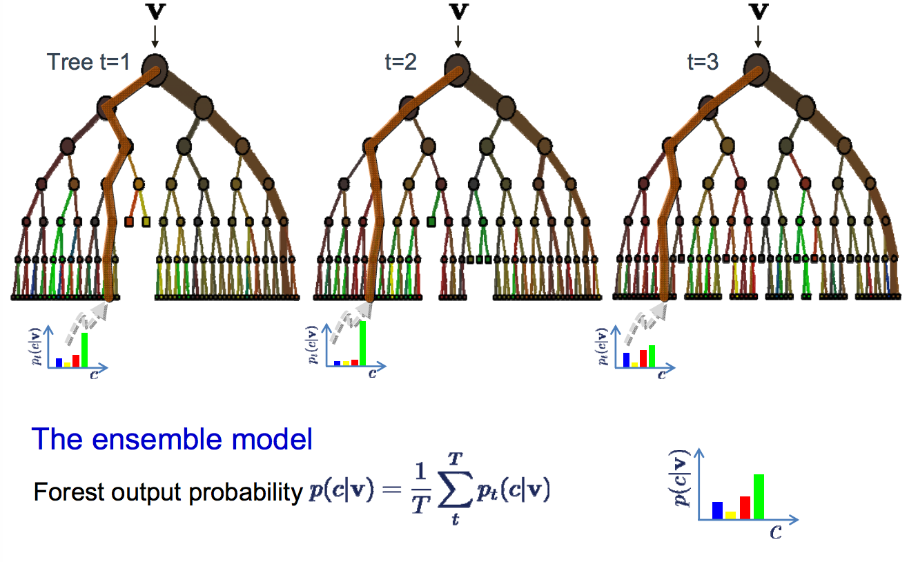
Random forest is just an improvement over the top of the decision tree algorithm. The core idea behind Random Forest is to generate multiple small decision trees from random subsets of the data (hence the name “Random Forest”).
Each of the decision tree gives a biased classifier (as it only considers a subset of the data). They each capture different trends in the data. This ensemble of trees is like a team of experts each with a little knowledge over the overall subject but thourough in their area of expertise.
Now, in case of classification the majority vote is considered to classify a class. In analogy with experts, it is like asking the same multiple choice question to each expert and taking the answer as the one that most no. of experts vote as correct. In case of Regression, we can use the avg. of all trees as our prediction.In addition to this, we can also weight some more decisive trees high relative to others by testing on the validation data.

Visualization:

  • Majority vote is taken from the experts (trees) for classification.
voting
  • We can also use probabilities and set the threshold for classification.
rf

Major hyperparameters in Random Forest

  1. ntree : Number of trees to grow in the forest. Typical values is around 100. More trees sometimes leads to overfitting.
  2. mtry : Number of variables randomly sampled as candidates at each split for a particular tree.
  3. replace: Sampling shoud be done with or without replacement.

Decision boundary in Random Forest:

As Random Forest uses ensemble of trees, it is capable of generating complex decision boundaries. Below are the kinds of decision boundaries that Random Forest can generate:

rf_boundary
rf_boundary

Top research paper writing service on Reddit. Get your paper done right the first time with the help of one of professional writers.

Random forest in R.

#Random Forest in R using IRIS data
#Split iris data to Training data and testing data

ind <- sample(2,nrow(iris),replace=TRUE)
train <- iris[ind==1,]
test <- iris[ind==2,]
head(train, 3)
##   Sepal.Length Sepal.Width Petal.Length Petal.Width Species
## 3          4.7         3.2          1.3         0.2  setosa
## 5          5.0         3.6          1.4         0.2  setosa
## 7          4.6         3.4          1.4         0.3  setosa
#Try plotting how a decision tree for IRIS will look like
x <- ctree(Species ~ ., data = iris)
plot(x, type = "simple")

#Train a RF model
model <- randomForest(Species~., data=train , ntree=50, mtry = 2,proximity=TRUE)

#Print RF model details
print(model)
## 
## Call:
##  randomForest(formula = Species ~ ., data = train, ntree = 50,      mtry = 2, proximity = TRUE) 
##                Type of random forest: classification
##                      Number of trees: 50
## No. of variables tried at each split: 2
## 
##         OOB estimate of  error rate: 6.41%
## Confusion matrix:
##            setosa versicolor virginica class.error
## setosa         25          0         0  0.00000000
## versicolor      0         24         2  0.07692308
## virginica       0          3        24  0.11111111
#Plot error vs ntree for classes
plot(model)

#Use the value of ntree where error becomes constant
#Plot variable importance matrix
varImpPlot(model)

#Test the model on testdata
pred <-predict(model , newdata=test)
table(pred, test$Species)
##             
## pred         setosa versicolor virginica
##   setosa         25          0         0
##   versicolor      0         23         1
##   virginica       0          1        22
#Plot the margin (positive ->  correct classification)

plot(margin(model,test$Species))

#Search for optimal value of mtry for random forest

tune <- tuneRF(iris[,-5],iris[,5])
## mtry = 2  OOB error = 5.33% 
## Searching left ...
## mtry = 1     OOB error = 5.33% 
## 0 0.05 
## Searching right ...
## mtry = 4     OOB error = 4.67% 
## 0.125 0.05


I highly encourage you to play with the hyperparameters for a while and see their effect on the output. ***

Pros and Cons?

Pros:

  • One of the most accurate decision models.
  • Works well on large datasets.
  • Can be used to extract variable importance.
  • Do not require feature engineering (scaling and normalization)

Cons:

  • Overfitting in case of noisy data.
  • Unlike decision trees, results are difficult to interpret.
  • Hyperparamters needs good tuning for high accuracy.

Applications

Random forests have successfully been implemented in a variety of fields. Some applications include:

  • Object recognition.
  • Molecular Biology (Analyzing amino acid sequences)
  • Remote sensing (Pattern recognition)
  • Astronomy (Star Galaxy classification, etc)

Additional resources:

I highly recommend you to go through the links below for an in-depth understanding of the Maths behind this algorithm.

  1. Random forest (University of British Columbia)
  2. Random forest Intuition

// add bootstrap table styles to pandoc tables
function bootstrapStylePandocTables() {
$(‘tr.header’).parent(‘thead’).parent(‘table’).addClass(‘table table-condensed’);
}
$(document).ready(function () {
bootstrapStylePandocTables();
});

(function () {
var script = document.createElement(“script”);
script.type = “text/javascript”;
script.src = “https://cdn.mathjax.org/mathjax/latest/MathJax.js?config=TeX-AMS-MML_HTMLorMML”;
document.getElementsByTagName(“head”)[0].appendChild(script);
})();