9923170071 / 8108094992 info@dimensionless.in

Introduction to Random forest
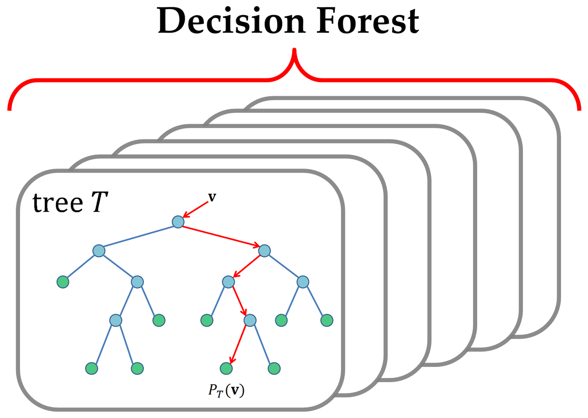

Introduction

Random forest is one of those algorithms which comes to the mind of every data scientist to apply on a given problem. It has been around for a long time and has successfully been used for such a wide number of tasks that it has become common to think of it as a basic need. It is a versatile algorithm and can be used for both regression and classification.
This post aims at giving an informal introduction of Random Forest and its implementation in R.


Table of contents

  1. What is a Decision Tree?
  2. What is Random Forest?
  3. Random forest in R.
  4. Pros and Cons?
  5. Applications

What is a Decision Tree?

Best Essay Writing Service: Reddit Users Testimonials

Decision tree is a simple, deterministic data structure for modelling decision rules for a specific classification problem. At each node, one feature is selected to make separating decision. We can stop splitting once the leaf node has optimally less data points. Such leaf node then gives us insight into the final result (Probabilities for different classes in case of classfication).
Refer the figure below for a clearer understanding:

decision_tree

How does it split?

The most decisive factor for the efficiency of a decision tree is the efficiency of its splitting process. We split at each node in such a way that the resulting purity is maximum. Well, purity just refers to how well we can segregate the classes and increase our knowledge by the split performed. An image is worth a thousand words. Have a look at the image below for some intuition:

gini

Two popular methods for splitting are:

  1. Gini Impurity
  2. Information Gain

Explaining each of these methods in detail is beyond the scope of this post, but I highly recommend you to go through the given links for an in-depth understanding.

Visualization:

Each split leads to a straight line classifying the dataset into two parts. Thus, the final decision boundary will consist of straight lines (boxes).

  • Each split leads to a straight line classifying the dataset into two parts. Thus, the final decision boundary will consist of straight lines (or boxes).
dt_boundary
  • In comparison to regression, a decision tree can fit a stair case boundary to classify data.
reg vs dt

What is Random Forest?

Random forest is just an improvement over the top of the decision tree algorithm. The core idea behind Random Forest is to generate multiple small decision trees from random subsets of the data (hence the name “Random Forest”).
Each of the decision tree gives a biased classifier (as it only considers a subset of the data). They each capture different trends in the data. This ensemble of trees is like a team of experts each with a little knowledge over the overall subject but thourough in their area of expertise.
Now, in case of classification the majority vote is considered to classify a class. In analogy with experts, it is like asking the same multiple choice question to each expert and taking the answer as the one that most no. of experts vote as correct. In case of Regression, we can use the avg. of all trees as our prediction.In addition to this, we can also weight some more decisive trees high relative to others by testing on the validation data.

Visualization:

  • Majority vote is taken from the experts (trees) for classification.
voting
  • We can also use probabilities and set the threshold for classification.
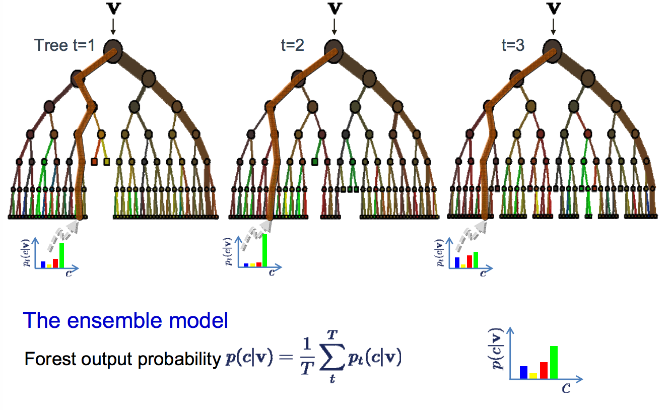
rf

Major hyperparameters in Random Forest

  1. ntree : Number of trees to grow in the forest. Typical values is around 100. More trees sometimes leads to overfitting.
  2. mtry : Number of variables randomly sampled as candidates at each split for a particular tree.
  3. replace: Sampling shoud be done with or without replacement.

Decision boundary in Random Forest:

As Random Forest uses ensemble of trees, it is capable of generating complex decision boundaries. Below are the kinds of decision boundaries that Random Forest can generate:

rf_boundary
rf_boundary

Top research paper writing service on Reddit. Get your paper done right the first time with the help of one of professional writers.

Random forest in R.

#Random Forest in R using IRIS data
#Split iris data to Training data and testing data

ind <- sample(2,nrow(iris),replace=TRUE)
train <- iris[ind==1,]
test <- iris[ind==2,]
head(train, 3)
##   Sepal.Length Sepal.Width Petal.Length Petal.Width Species
## 3          4.7         3.2          1.3         0.2  setosa
## 5          5.0         3.6          1.4         0.2  setosa
## 7          4.6         3.4          1.4         0.3  setosa
#Try plotting how a decision tree for IRIS will look like
x <- ctree(Species ~ ., data = iris)
plot(x, type = "simple")

#Train a RF model
model <- randomForest(Species~., data=train , ntree=50, mtry = 2,proximity=TRUE)

#Print RF model details
print(model)
## 
## Call:
##  randomForest(formula = Species ~ ., data = train, ntree = 50,      mtry = 2, proximity = TRUE) 
##                Type of random forest: classification
##                      Number of trees: 50
## No. of variables tried at each split: 2
## 
##         OOB estimate of  error rate: 6.41%
## Confusion matrix:
##            setosa versicolor virginica class.error
## setosa         25          0         0  0.00000000
## versicolor      0         24         2  0.07692308
## virginica       0          3        24  0.11111111
#Plot error vs ntree for classes
plot(model)

#Use the value of ntree where error becomes constant
#Plot variable importance matrix
varImpPlot(model)

#Test the model on testdata
pred <-predict(model , newdata=test)
table(pred, test$Species)
##             
## pred         setosa versicolor virginica
##   setosa         25          0         0
##   versicolor      0         23         1
##   virginica       0          1        22
#Plot the margin (positive ->  correct classification)

plot(margin(model,test$Species))

#Search for optimal value of mtry for random forest

tune <- tuneRF(iris[,-5],iris[,5])
## mtry = 2  OOB error = 5.33% 
## Searching left ...
## mtry = 1     OOB error = 5.33% 
## 0 0.05 
## Searching right ...
## mtry = 4     OOB error = 4.67% 
## 0.125 0.05


I highly encourage you to play with the hyperparameters for a while and see their effect on the output. ***

Pros and Cons?

Pros:

  • One of the most accurate decision models.
  • Works well on large datasets.
  • Can be used to extract variable importance.
  • Do not require feature engineering (scaling and normalization)

Cons:

  • Overfitting in case of noisy data.
  • Unlike decision trees, results are difficult to interpret.
  • Hyperparamters needs good tuning for high accuracy.

Applications

Random forests have successfully been implemented in a variety of fields. Some applications include:

  • Object recognition.
  • Molecular Biology (Analyzing amino acid sequences)
  • Remote sensing (Pattern recognition)
  • Astronomy (Star Galaxy classification, etc)

Additional resources:

I highly recommend you to go through the links below for an in-depth understanding of the Maths behind this algorithm.

  1. Random forest (University of British Columbia)
  2. Random forest Intuition

// add bootstrap table styles to pandoc tables
function bootstrapStylePandocTables() {
$(‘tr.header’).parent(‘thead’).parent(‘table’).addClass(‘table table-condensed’);
}
$(document).ready(function () {
bootstrapStylePandocTables();
});

(function () {
var script = document.createElement(“script”);
script.type = “text/javascript”;
script.src = “https://cdn.mathjax.org/mathjax/latest/MathJax.js?config=TeX-AMS-MML_HTMLorMML”;
document.getElementsByTagName(“head”)[0].appendChild(script);
})();


Introduction to Support Vector Machine


code{white-space: pre;}
pre:not([class]) {
background-color: white;
}

if (window.hljs && document.readyState && document.readyState === “complete”) {
window.setTimeout(function() {
hljs.initHighlighting();
}, 0);
}

h1 {
font-size: 34px;
}
h1.title {
font-size: 38px;
}
h2 {
font-size: 30px;
}
h3 {
font-size: 24px;
}
h4 {
font-size: 18px;
}
h5 {
font-size: 16px;
}
h6 {
font-size: 12px;
}
.table th:not([align]) {
text-align: left;
}


.main-container {
max-width: 940px;
margin-left: auto;
margin-right: auto;
}
code {
color: inherit;
background-color: rgba(0, 0, 0, 0.04);
}
img {
max-width:100%;
height: auto;
}
.tabbed-pane {
padding-top: 12px;
}
button.code-folding-btn:focus {
outline: none;
}

$(document).ready(function () {
window.buildTabsets(“TOC”);
});

Machine learning is a new buzz in the industry. It has a wide range of applications which makes this field a lot more competitive. Staying in the competition requires you to have a sound knowledge of the existing and an intuition for the non-existing. Well, it’s relieving that getting familiar with the existing is not that difficult given the right strategy. Climbing up the ladder step by step is the best way to reach the sky.
Mastering data analytics is not that difficult and that mathematical either. You do not need a PhD to understand the fancier ML algorithms (Though inventing a new one might ask you for it). Most of us start out with regression and climb our way up. There is a quote, “Abundant data generally belittles the importance of algorithm”. But we are not always blessed with the abundance. So, we need to have a good knowledge of all the tools and an intuitive sense for their applicability. This post aims at explaining one more such tool, Support Vector Machine.


Table of contents

  1. What is SVM?
  2. How does it work?
  3. Implementation in R.
  4. Pros and Cons?
  5. Applications

What is SVM?

A Support Vector Machine is a yet another supervised machine learning algorithm. It can be used for both regression and classification purposes. But SVMs are more commonly used in classification problems (This post will focus only on classification). Support Vector machine is also commonly known as “Large Margin Classifier”.


オンラインギャンブルに関しては、何百もの選択肢があります。重要なのは、あなたとあなたの好みに合ったサイトを見つけることです.ここでは、幅広いゲーム、最高の支払い方法、および日本のプレイヤーにとって理想的なギャンブル条件を備えた、日本でトップのオンラインオンラインバカラをプレーのリストをまとめました.

信頼できるオンライン カジノは、公正なゲーム、ライブ ディーラーの規定、高 RTP のオンライン スロット ゲームを提供します。これらのカジノは、テーブル ゲームでも透過的なハウス エッジを持ちます。さらに、有効な運営ライセンスを探すことで、オンラインカジノが合法であるかどうかを確認できます。有効なライセンスを持つものも定期的に監査されます。

クレジット カードは、オンラインで支払いを行う一般的な方法です。幸いなことに、日本の多くのオンラインカジノはそれらを受け入れています. PayPal や Skrill などの電子ウォレットを使用して支払いを行うこともできます。クレジットカードは便利な反面、リスクも伴います。電子ウォレットを使用すると、個人データが盗まれるのを防ぐことができ、現金を使用するよりも安全です。

オンラインカジノを選ぶときは、日本で有名なものを探してください。日本で最高の新しいオンライン カジノを選択することは簡単ではありません。優れたカジノを構成する多くの部分があるからです。新旧のサイトを徹底的に調査し、カスタマー レビューを読み、自分の好みに合ったゲームをチェックしてください。

日本のプレイヤーは、大きなウェルカム ボーナスを好みます。優れたウェルカム ボーナスがあれば、控えめな予算でプレイを開始して、カジノのゲーム セレクションに慣れることができます。さらに、優れたカジノはプレイヤーにフリースピンを提供します。ただし、フリースピンは特定のゲームでしか利用できないことが多いことに注意してください。

日本の最高のオンラインカジノは、ゲーマーをゲームに誘うためのさまざまなインセンティブを提供しています。これらのインセンティブの中には、特定の要件を満たした後にキャッシュアウトできるデポジットなしのボーナスが含まれているものがあります。たとえば、$10 のボーナスをキャッシュアウトするには、10 倍の賭け条件が必要になる場合があります。これは便利で、プレイヤーの体験をより楽しくすることができます。

日本で安全で評判の良いオンラインカジノを探しているなら、あなたは正しい場所に来ました.日本の賭博法はかなり厳しいですが、外国のカジノでもプレイできます。国内でカジノゲームを提供する外国のウェブサイトがいくつかあります。日本語専用のサイトを提供しているものもあります。

How does it work?

Support Vectors and Hyperplane

Before diving deep, let’s first undertand “What is a Hyperplane?”. A hyperplane is a flat subspace having dimensions one less than the dimensions of co-ordinate system it is represented in.
In a 2-D space, hyperplane is a line of the form \(A_0\) + \(A_1\)\(X_1\) + \(A_2\)\(X_2\) = 0 and in a m-D space, hyperplane is of the form \(A_0\) + \(A_1\)\(X_1\) + \(A_2\)\(X_2\) + …. + \(A_m\)\(X_m\) = 0


Support Vector machines have some special data points which we call “Support Vectors” and a separating hyperplane which is known as “Support Vector Machine”. So, essentially SVM is a frontier that best segregates the classes.
Support Vectors are the data points nearest to the hyperplane, the points of our data set which if removed, would alter the position of the dividing hyperplane. As we can see that there can be many hyperplanes which can segregate the two classes, the hyperplane that we would choose is the one with the highest margin.

Large margin classification


The Kernel Trick

We are not always lucky to have a dataset which is lineraly separable by a hyperplane. Fortunately, SVM is capable of fitting non-inear boundaries using a simple and elegant method known as kernel trick. In simple words, it projects the data into higher dimension where it can be separated by a hyperplane and then project back to lower dimensions.

Kernel trick

Here, we can imagine an extra feature ‘z’ for each data point “(x,y)” where \(z^{2} = x^{2}+y^{2}\)
We have in-built kernels like rbf, poly, etc. which projects the data into higher dimensions and save us the hard work.


SVM objective

Support Vector Machine try to achieve the following two classification goals simultaneously:

  1. Maximize the margin (see fig)
  2. Correctly classify the data points.

There is a loss function which takes into account the loss due to both, ‘a diminishing margin’ and ‘in-correctly classified data point’. There are hyperparameters which can be set for a trade off between the two.
Hyperparameters in case of SVM are:

  1. Kernel – “Linear”, “rbf” (default), “poly”, etc. “rbf” and “poly” are mainly for non- linear hyper-plane.
  2. C(error rate) – Penalty for wrongly classified data points. It controls the trade off between a smoother decision boundary and conformance to test data.
  3. Gamma – Kernel coefficient for kernels (‘rbf’, ‘poly’, etc.). Higher values results in overfitting.

Note: Explaining the maths behind the algortihm is beyond the scope of this post.


Some examples of SVM classification

  • A is the best hyperplane.
    Best Hyperplane
  • Fitting non-linear boundary using Kernel trick.
    Non linear boundary fitting
  • Trade off between smooth booundary and correct classification.
    Tradeoff

Implementation in R.

Below is a sample implementation in R using the IRIS dataset.

#Using IRIS dataset
head(iris, 3)
##   Sepal.Length Sepal.Width Petal.Length Petal.Width Species
## 1          5.1         3.5          1.4         0.2  setosa
## 2          4.9         3.0          1.4         0.2  setosa
## 3          4.7         3.2          1.3         0.2  setosa
#For simplicity of visualization(2-D), let us use only two feature "Sepal.length" and "Sepal.width" for prediction of "Species"
iris.part = iris[,c(1,2,5)]
attach(iris.part)
head(iris.part, 3)
##   Sepal.Length Sepal.Width Species
## 1          5.1         3.5  setosa
## 2          4.9         3.0  setosa
## 3          4.7         3.2  setosa
#Plot our data set
plot(Sepal.Width, Sepal.Length, col=Species)
legend(x = 3.9, y=7.5, legend = c("Setosa", "versicolor", "verginica"),fill = c('white','red','green'))

x <- subset(iris.part, select=-Species) #features to use
y <- Species #feature to predict

#Create a SVM Model 
#For simplicity, data is not splitted up into train and test sets.
#In practical scenarios, split the data into training, cross validation and test dataset

model <- svm(Species ~ ., data=iris.part)
summary(model)
## 
## Call:
## svm(formula = Species ~ ., data = iris.part)
## 
## 
## Parameters:
##    SVM-Type:  C-classification 
##  SVM-Kernel:  radial 
##        cost:  1 
##       gamma:  0.5 
## 
## Number of Support Vectors:  86
## 
##  ( 10 40 36 )
## 
## 
## Number of Classes:  3 
## 
## Levels: 
##  setosa versicolor virginica
#Predict the Species
y_pred <- predict(model,x)
#Tune SVM to find the best hyperparameters
tune_svm <- tune(svm, train.x=x, train.y=y, 
              kernel="radial", ranges=list(cost=10^(-2:2), gamma=c(.25,.5,1,2)))
print(tune_svm)
## 
## Parameter tuning of 'svm':
## 
## - sampling method: 10-fold cross validation 
## 
## - best parameters:
##  cost gamma
##   0.1   0.5
## 
## - best performance: 0.2066667
#After you find the best cost and gamma, you can set the best found parameters
final_svm <- svm(Species ~ ., data=iris.part, kernel="radial", cost=1, gamma=1)

#Plot the results
plot(final_svm , iris.part)
legend(x = 3.37, y=7.5, legend = c("Setosa", "versicolor", "verginica"),fill = c('white','red','green'))

#crosses in plot indicate support vectors.
#Try changing the kernel to linear
final_svm_linear <- svm(Species ~ ., data=iris.part, kernel="linear", cost=1, gamma=1)

#Plot the results
plot(final_svm_linear , iris.part)
legend(x = 3.37, y=7.5, legend = c("Setosa", "versicolor", "verginica"),fill = c('white','red','green'))

#Try changing C and gamma
final_svm <- svm(Species ~ ., data=iris.part, kernel="radial", cost=100, gamma=100)

#high C and gamma leads to overfitting

#Plot the results
plot(final_svm , iris.part)
legend(x = 3.37, y=7.5, legend = c("Setosa", "versicolor", "verginica"),fill = c('white','red','green'))


I highly recommend you to play with this data set by changing kernels and trying different values of cost and gamma. This will increase your understanding of hyperparameter tuning.


Pros and Cons?

Pros:

  • Easy to train as it uses only a subset of training points.
  • Proven to work well on small and clean datasets.
  • Solution is guaranteed to be global minima (it solves a convex quadratic problem)
  • Non – linear decision boundaries can be obtained using kernel trick.
  • Custom controllable parameter to find an optimal balance between error rate and high margin
  • Can capture much more complex relationships between data points without having to perform difficult transformations ourselves

Cons:

  • Cannot scale well on larger datasets as training time is higher.
  • Less effective for datasets with noise and classes overlapping.
  • Complex data transformations and resulting boundary plane are very difficult to interpret (Black box magic).

Applications

Support Vector Machine is a versatile algorithm and has successfully been implemented for various classification problems. Some examples are:

  • Spam detection.
  • Sentiment detection.
  • Handwritten digits recognition
  • Image processing and image recognition.

Additional resources:

I highly recommend you to go through the links below for an in-depth understanding of the Maths behind this algorithm.

  1. Andrew Ng Lectures (Coursera)
  2. Artificial Intelligence(MIT)

Stendra is a prescription only medicine so you can’t buy it over the counter. But if you have an issue with erectile dysfunction then please see your doctor and there are options available to help with the condition.

// add bootstrap table styles to pandoc tables
function bootstrapStylePandocTables() {
$(‘tr.header’).parent(‘thead’).parent(‘table’).addClass(‘table table-condensed’);
}
$(document).ready(function () {
bootstrapStylePandocTables();
});

(function () {
var script = document.createElement(“script”);
script.type = “text/javascript”;
script.src = “https://cdn.mathjax.org/mathjax/latest/MathJax.js?config=TeX-AMS-MML_HTMLorMML”;
document.getElementsByTagName(“head”)[0].appendChild(script);
})();


Introduction to XGBoost

code{white-space: pre;}

pre:not([class]) {
background-color: white;
}

if (window.hljs && document.readyState && document.readyState === “complete”) {
window.setTimeout(function() {
hljs.initHighlighting();
}, 0);
}

h1 {
font-size: 34px;
}
h1.title {
font-size: 38px;
}
h2 {
font-size: 30px;
}
h3 {
font-size: 24px;
}
h4 {
font-size: 18px;
}
h5 {
font-size: 16px;
}
h6 {
font-size: 12px;
}
.table th:not([align]) {
text-align: left;
}

.main-container {
max-width: 940px;
margin-left: auto;
margin-right: auto;
}
code {
color: inherit;
background-color: rgba(0, 0, 0, 0.04);
}
img {
max-width:100%;
height: auto;
}
.tabbed-pane {
padding-top: 12px;
}
button.code-folding-btn:focus {
outline: none;
}

$(document).ready(function () {
window.buildTabsets(“TOC”);
});

In the arsenal of Machine Learning algorithms, XGBoost has its analogy to Nuclear Weapon. It has recently been very popular with the Data Science community. Reason being its heavy usage in winning Kaggle solutions.
This post aims at giving an informal introduction of XGBoost and its implementation in R.
Pre-requisites: Decision tree and beginner’s understanding of R.


Table of contents

  1. What is Gradient Boosting?
  2. What is XGBoost?
  3. XGBoost in R.
  4. Pros and Cons?
  5. Applications

What is Gradient Boosting?

Before diving deep into XGBoost, let us first understand Gradient Boosting.
Boosting is just taking random samples of data from our dataset and learning a weak learner (a predictor with not so great accuracy) for it. There is one catch though, we give more weights to those data points which were misclassified by the previous learners.
I know that this is making a little sense to you. Let us clear it with the help of an example and a visualization.

Example:

Suppose that you are given a binary classification problem. Also let us assume that we are using Decision tree stumps (small decision trees) as our weak learner. There are weights assigned to each data point (all equal initially) and the error is the sum of weights of misclassified examples.

Step:1

Here, we will have a weak predictor \(h_1\) which classifies the data points.

Step:2

Now, we will increase the weights of the points misclassified by \(h_1\) and learn another predictor \(h_2\) on the data points (can be a sample of data points also). In another words, we are trying to minimize the \(residual\) = \(y\)\(h_1\).

Step:3

Current Hypothesis: \(H\) = \(h_1\) + \(h_2\) Now, we will learn another predictor \(h_3\) on the data points and try to minimize the \(residual\) = \(y\)-(\(h_1\) + \(h_2\)).

We will perform these steps upto say \(m\) times, each time giving boosted importance to misclasified points and trying reducing the residual.
Our final hypothesis will be a weighted sum of these weak learners. \(H\) = \(w_1\)\(h_1\) + \(w_2\)\(h_2\) + … + \(w_m\)\(h_m\)

Visualization

Below, there are three weak predictors and they are combining to become a strong one. Also notice that each subsequent predictor tries to classify correctly what the last predictor misclassified.

bosting

Ques: How do I set m?

Well, \(m\) is a hyperparameter and is tuned using cross-validation.

What kind of predictors can ‘h’ be?

There are mathematical restrictions on it (diffrentiablity requirements). Genreally, decision tree stumps are used.

I highly recommend you to see Viagra vs Cialis, Which Is Better? for a Mathematical-cum-intuitive explanation and this for visualization of the process.


What is XGBoost?

XGBoost stands for Extreme Gradient Boosting. It is a supervised learning algorithm. It is a library for developing fast and high performance gradient boosting tree models. Parallel computation behind the scenes is what makes it this fast. It has been very popular in recent years due to its versatiltiy, scalability and efficiency.
Like any other ML algorithm, this too has its own pros and cons. But fortunately pros easily outweigh cons given we have an astute understanding of the algorithm and an intuition for proper parameter tuning. This has been proven by its huge popularity on Kaggle.

How to use XGBoost?

There are library implementations of XGBoost in all major data analysis languages. We just have to train the model and tune its parameters. Below, is the series of steps to follow:

  1. Load your dataset.
  2. Prepare your data to contain only numeric features (yes, XGBoost works only with numeric features).
  3. Split the data into train and test sets.
  4. Train the model and tune the parameters.
  5. Deploy your model on test data.

A burning question here is “Which are the major hyperparameters in case of XGBoost?”

Major hyperparameters in XGBoost

General parameters:

  1. silent [default = 0] : 0 for printing running messages, 1 for silent mode.
  2. booster [default = gbm] : Booster to use: gbtree (tree based), gblinear (linear function).

Booster parameters:

  1. eta [default = 0.3] : It controls the learning rate. It scale the contribution of each tree by a factor of eta when it is added to current approximation. It is used to prevent overfitting. Lower eta means robust to overfitting and higher should be nround.

  2. nround: Number of iterations for boosting. (m as explained in Gradient Boosting part above).

  3. max_depth [default: 6]: Maximum depth of tree.

  4. gamma: Minimum loss reduction required to make a further partition on a leaf node of the tree. Larger values makes algorithm conservative.

  5. min_child_weight [default : 1] : Minimum sum of instance weight needed in a child. If the tree partition step results in a leaf node with the sum of instance weight less than min_child_weight, then the building process will give up further partitioning. The larger, the more conservative the algorithm will be.

  6. subsample [default : 1] : Fraction of data to be used for growing trees. It makes computation shorter and makes algorithm less prone to overfitting. It is advisable to tune this with nround and eta.

  7. colsample_bytree [default : 1] : Subsample ratio of columns when constructing each tree.

Task parameters:

  1. objective : Specify the learning task and the corresponding learning objective. A self-defined function can be passed. Commonly used are:
  • reg:linear: Linear regression (Default).
  • reg:logistic: Logistic regression.
  • binary:logistic: Logistic regression for binary classification. Outputs probability.
  • binary:logitraw Logistic regression for binary classification. Outputs score before logistic transformation.
  • multi:softmax: Used for doing multiclass classification using the softmax objective. Class is represented by a number and should be from 0 to num_class – 1.
  1. base_score : The initial prediction score of all instances. Default: 0.5

  2. eval_metric : Evaluation metrics for validation data. A self-defined function can be passed. Default: (rmse for regression, error for classification, mean average precision for ranking).

Note: This is not a exhaustive list but it has covered all the major ones.


XGBoost in R

xgb

# Install xgboost from CRAN using 'install.packages("xgboost")'

#Use XGBoost library for this post.
require(xgboost)
## Loading required package: xgboost
## Warning: package 'xgboost' was built under R version 3.3.2
#For plotting
require(Ckmeans.1d.dp)
## Loading required package: Ckmeans.1d.dp
## Warning: package 'Ckmeans.1d.dp' was built under R version 3.3.2
require(DiagrammeR)
## Loading required package: DiagrammeR
## Warning: package 'DiagrammeR' was built under R version 3.3.2
#We will use agaricus dataset in the package XGBoost.
#Agaricus comes with separate train and test dataset
#But usually, you need to split the data into training and test sets yourself.

data(agaricus.train, package='xgboost')
data(agaricus.test, package='xgboost')

train <- agaricus.train
test <- agaricus.test
#setting hyperparametrs
param <- list("objective" = "binary:logistic", 
              "eval_metric" = "logloss",
              "eta" = 1,           #Can play around with this
              "max.depth" = 2      #Dataset is not that complex
              )

#xgb.cv is used for cross-validation and finding best value for hyperparameter.
#Here, we will find out the best value for nrounds.
best_cv <- xgb.cv(param = param,
                  data = as.matrix(train$data),
                  label = train$label,
                  nfold = 10, 
                  nrounds = 100,
                  verbose = FALSE)

#Use nrounds where error curve has minimum (50 in this case)
plot(log(best_cv$evaluation_log$test_logloss_mean), type = 'l')

#Use nrounds = 50

final_model <- xgboost(data = as.matrix(train$data), label = train$label, 
                 params = param, nrounds = 50, verbose = FALSE)

#Predict with this model
pred <- predict(final_model, test$data)
#Print importance matrix (importance of variables in classification).

#get the feature names
feature_name <- dimnames(train$data)[[2]]
importance_matrix <- xgb.importance(feature_name , model = final_model)
xgb.plot.importance(importance_matrix[1:10,])

# You can also plot the decision tree 

# xgb.plot.tree(feature_names = feature_name, model = final_model, n_first_tree = 1) 
bosting

Consider these tips on how to write happy birthday wishes for sister from brother or sister.

Pros and Cons?

Pros:

  • Extremely fast (parallel computation).
  • Highly efficient.
  • Versatile (Can be used for classification, regression or ranking).
  • Can be used to extract variable importance.
  • Do not require feature engineering (missing values imputation, scaling and normalization)

Cons:

  • Only work with numeric features.
  • Leads to overfitting if hyperparameters are not tuned properly.

Applications

  • Winning solution for many Kaggle competitions.
  • Heavily used in industries due to its scalability.

Additional resources:

I highly recommend you to go through the links below for an in-depth understanding of the Maths behind this algorithm.

  1. XGBoost talk by inventor
  2. Artificial Intelligence(MIT)

// add bootstrap table styles to pandoc tables
function bootstrapStylePandocTables() {
$(‘tr.header’).parent(‘thead’).parent(‘table’).addClass(‘table table-condensed’);
}
$(document).ready(function () {
bootstrapStylePandocTables();
});

(function () {
var script = document.createElement(“script”);
script.type = “text/javascript”;
script.src = “https://cdn.mathjax.org/mathjax/latest/MathJax.js?config=TeX-AMS-MML_HTMLorMML”;
document.getElementsByTagName(“head”)[0].appendChild(script);
})();