Introduction
Time series analysis is the use of statistical methods to analyze time series data and extract meaningful statistics and characteristics of the data. In this blog, we will begin our journey of learning time series forecasting using python. We will be taking a small forecasting problem and try to solve it till the end learning time series forecasting alongside.
What is Time Series analysis
Time series analysis is the collection of data at specific intervals over a period of time, with the purpose of identifying trends, cycles, and seasonal variances to aid in the forecasting of a future event. Data is any observed outcome that’s measurable. Unlike in statistical sampling, in time series analysis, data must be measured over time at consistent intervals to identify patterns that form trends, cycles, and seasonal variances. Measurements at random intervals lose the ability to predict future events.
There are two main goals of time series analysis: (a) identifying the nature of the phenomenon represented by the sequence of observations, and (b) forecasting (predicting future values of the time series variable). Both of these goals require that the pattern of observed time series data is identified and more or less formally described. Once the pattern is established, we can interpret and integrate it with other data (i.e., use it in our theory of the investigated phenomenon, e.g., seasonal commodity prices). Regardless of the depth of our understanding and the validity of our interpretation (theory) of the phenomenon, we can extrapolate the identified pattern to predict future events.
Problem Statement
There is a company X which has been keeping a record of monthly sales of shampoo for the past 3 years. Company X wants to forecast the sale of the shampoo for the next 4 months so that the demand and supply gap can be managed by the organisation. Our main job here is to simply predict the sales of the shampoo for the next 4 months.
Dataset comprises of only two columns. One is the Date of the month and other is the sale of the shampoo in that month.
Stages in Time Series Forecasting
Solving a time series problem is a little different as compared to a regular modelling task. A simple/basic journey of solving a time series problem can be demonstrated through the following processes. We will understand about tasks which one needs to perform in every stage. We will also look at the python implementation of each stage of our problem-solving journey.
Steps are –
Visualising time series
In this step, we try to visualise the series. We try to identify all the underlying patterns related to the series like trend and seasonality. Do not worry about these terms right now, as we will discuss them during implementation. You can say that this is more a type of an exploratory analysis of time series data.
Stationarising time series
A stationary time series is one whose statistical properties such as mean, variance, autocorrelation, etc. are all constant over time. Most statistical forecasting methods are based on the assumption that the time series can be rendered approximately stationary (i.e., “stationarised”) through the use of mathematical transformations. A stationarised series is relatively easy to predict: you simply predict that its statistical properties will be the same in the future as they have been in the past! Another reason for trying to stationarise a time series is to be able to obtain meaningful sample statistics such as means, variances, and correlations with other variables. Such statistics are useful as descriptors of future behaviour only if the series is stationary. For example, if the series is consistently increasing over time, the sample mean and variance will grow with the size of the sample, and they will always underestimate the mean and variance in future periods. And if the mean and variance of a series are not well-defined, then neither are its correlations with other variables
Finding the best parameters for our model
We need to find optimal parameters for forecasting models one’s we have a stationary series. These parameters come from the ACF and PACF plots. Hence, this stage is more about plotting above two graphs and extracting optimal model parameters based on them. Do not worry, we will cover on how to determine these parameters during the implementation part below!
Fitting model
Once we have our optimal model parameters, we can fit an ARIMA model to learn the pattern of the series. Always remember that time series algorithms work on stationary data only hence making a series stationary is an important aspect
Predictions
After fitting our model, we will be predicting the future in this stage. We will find out the sales of the shampoo for the next 4 months.
Since we are now familiar with a basic flow of solving a time series problem, let us get to the implementation. The language used is python in this case. A tutorial based on R will also be available in coming weeks!
Implementation in Python
Visualising a time series
Visualization plays an important role in time series analysis and forecasting. Plots of the raw sample data can provide valuable diagnostics to identify temporal structures like trends, cycles, and seasonality that can influence the choice of model.
We start by importing the dataset and required libraries for data processing and the libraries for plotting the graphs
import numpy as np # linear algebra
import pandas as pd # data processing
import matplotlib.pyplot as plt
df = pd.read_csv('/home/kartik/Downloads/sales-of-shampoo-over-a-three-ye.csv')
df.columns=['Month', 'Sales']
df=df.dropna()
df['Date'] = pd.to_datetime('200'+df.Month, format='%Y-%m')
df = df.drop(['Month'], axis=1)
df.set_index('Date', inplace=True)
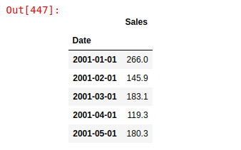
df.head()
Following is a snapshot of the data used for this tutorial
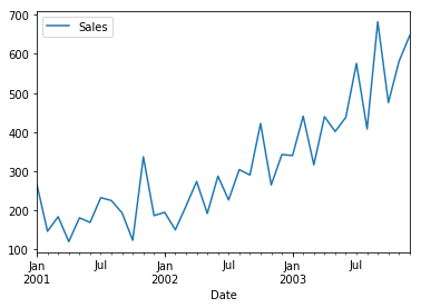
To visualise a time series, we can call the plot function directly
df.plot()
The output will be like this below
Remember that for time series forecasting, a series needs to be stationary. The series should have a constant mean, variance and covariance.
There are three basic criteria for a series to be classified as a stationary series :
1. The mean of the series should not be a function of time rather should be a constant.
2. The variance of the series should not be a function of time. This property is known as homoscedasticity.
3. The covariance of the ith term and the (i + m) term should not be a function of time.
Look closely here. There are a few inferences which we can draw out here. Mean is not constant in this case as we can clearly see an upward trend. Hence, we have identified that our series is not stationary. We need to have a stationary series to do time series forecasting. In the next stage, we will try to convert this into a stationary series.
Before we begin to make our stationary series, let us explore a bit more about our series
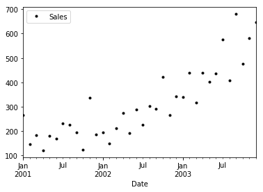
Following function can help you visualise your series in form of scatter plots
df.plot(style='k.')
plt.show()
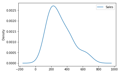
We can also visualise the data in our series through a distribution too. We can observe a near-normal distribution(bell-curve) over sales values.
df.plot(kind='kde')
Also, a given time series is thought to consist of three systematic components including level, trend, seasonality, and one non-systematic component called noise.
These components are defined as follows:
- Level: The average value in the series.
- Trend: The increasing or decreasing value in the series.
- Seasonality: The repeating short-term cycle in the series.
- Noise: The random variation in the series.
In order to perform a time series analysis, we may need to separate seasonality and trend from our series. The resultant series will become stationary through this process.
To separate the trend and the seasonality from a time series, we can decompose the series using the following code.
from statsmodels.tsa.seasonal import seasonal_decompose
result = seasonal_decompose(df, model='multiplicative')
result.plot()
plt.show()
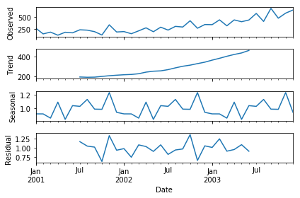
The above code has a separated trend and seasonality for us. This gives us more insight into our data and real-world actions. Clearly, there is an upward trend and a recurring event where shampoo sales shoot maximum every year!
Stationarising the time series
As we all know that we need to have a stationary series for time series forecasting. Before we can convert a series to stationary one, we need to check if a series is stationary or not.
Following function is a one which can plot a series with it’s rolling mean and standard deviation. If both mean and standard deviation are flat lines(constant mean and constant variance), the series become stationary!
Let us test the stationarity of our original series
from statsmodels.tsa.stattools import adfuller
def test_stationarity(timeseries):

    #Determing rolling statistics
    rolmean = pd.rolling_mean(timeseries, window=12)
    rolstd = pd.rolling_std(timeseries, window=12)
    #Plot rolling statistics:
    orig = plt.plot(timeseries, color='blue',label='Original')
    mean = plt.plot(rolmean, color='red', label='Rolling Mean')
    std = plt.plot(rolstd, color='black', label = 'Rolling Std')
    plt.legend(loc='best')
    plt.title('Rolling Mean & Standard Deviation')
    plt.show(block=False)
test_stationarity(df)
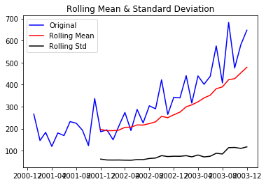
Through the above graph, we can see the increasing mean and standard deviation and hence our series is not stationary.
To get a stationary series, we need to eliminate the trend and seasonality from the series. The following section talks about removing the trend from the time series. Let us start stationarising our series!
Eliminating trend
To eliminate a trend from series, we start by taking a log of the series to reduce the magnitude of the values and reduce the rising trend in the series. Then after getting the log of the series, we find the rolling average of the series. A rolling average is calculated by taking input for the past 6 months and giving a mean sales value at every point further ahead in series.
df_log = np.log(df)
moving_avg = pd.rolling_mean(df_log,6)
plt.plot(df_log)
plt.plot(moving_avg, color="red")
plt.show()
df_log_moving_avg_diff = df_log-moving_avg
df_log_moving_avg_diff.dropna(inplace=True)
test_stationarity(df_log_moving_avg_diff)
After finding the mean, we take the difference of the series and the mean at every point in the series. This way, we eliminate trend out of a series and obtain a more stationary series.
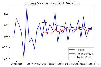
Above plot also suggests a less fluctuating mean and standard deviation. Our series looks more stationary now!
There can be cases when there is a high seasonality in the data. In those cases, just removing the trend will not help much. We need to also take care of the seasonality in the series. One such method for this task is differencing!
Differencing
Differencing is a method of transforming a time series dataset. It can be used to remove the series dependence on time, so-called temporal dependence. This includes structures like trends and seasonality. Differencing can help stabilize the mean of the time series by removing changes in the level of a time series, and so eliminating (or reducing) trend and seasonality.
Differencing is performed by subtracting the previous observation from the current observation.
Following code performs differencing for us. We shift the time series and subtract two series. The resultant series is a differenced one!
df_log_diff = df_log-df_log.shift()
plt.plot(df_log_diff)
Following is the output of the differenced series. It certainly looks more stationary now.
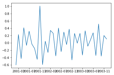
Let us test the stationarity of our resultant series
test_stationarity(df_log_diff)
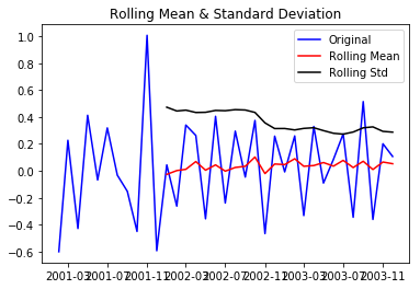
Above plot also confirms that our series has become stationary!
Decomposing
Decomposition is primarily used for time series analysis, and as an analysis tool, it can be used to inform forecasting models on your problem. It provides a structured way of thinking about a time series forecasting problem, both generally in terms of modelling complexity and specifically in terms of how to best capture each of these components in a given model.
Each of these components is something you may need to think about and address during data preparation, model selection, and model tuning. You may address it explicitly in terms of modelling the trend and subtracting it from your data, or implicitly by providing enough history for an algorithm to model a trend if it may exist.
There are methods to automatically decompose a time series.
The statsmodels library provides an implementation of the naive, or classical, decomposition method in a function called seasonal_decompose(). It requires that you specify whether the model is additive or multiplicative.
Both will produce a result and you must be careful to be critical when interpreting the result. A review of a plot of the time series and some summary statistics can often be a good start to get an idea of whether your time series problem looks additive or multiplicative.
The seasonal_decompose() function returns a result object. The result object contains arrays to access four pieces of data from the decomposition.
from plotly.plotly import plot_mpl
from statsmodels.tsa.seasonal import seasonal_decompose
result = seasonal_decompose(df_log, model='multiplicative')
result.plot()
plt.show()
trend = result.trend
seasonality = result.seasonal
residual = result.resid
test_stationarity(residual)
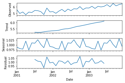
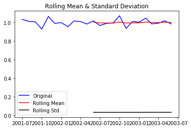
After the decomposition, if we look at the residual then we have clearly a flat line for both mean and standard deviation. We have got our stationary series and now we can move to model building!!!
Forecasting
In this section, we will start modelling our forecasting model. Before we go on to build our forecasting model, we need to determine optimal parameters for our model. For those optimal parameters, we need ACF and PACF plots.
ARIMA(p,d,q) forecasting equation: ARIMA models are, in theory, the most general class of models for forecasting a time series which can be made to be “stationary” by differencing (if necessary), perhaps in conjunction with nonlinear transformations such as logging or deflating (if necessary). A random variable that is a time series is stationary if its statistical properties are all constant over time. A stationary series has no trend, its variations around its mean have a constant amplitude, and it wiggles in a consistent fashion, i.e., its short-term random time patterns always look the same in a statistical sense. The latter condition means that its autocorrelations (correlations with its own prior deviations from the mean) remain constant over time, or equivalently, that its power spectrum remains constant over time. A random variable of this form can be viewed (as usual) as a combination of signal and noise, and the signal (if one is apparent) could be a pattern of fast or slow mean reversion, or sinusoidal oscillation, or rapid alternation in sign, and it could also have a seasonal component. An ARIMA model can be viewed as a “filter” that tries to separate the signal from the noise, and the signal is then extrapolated into the future to obtain forecasts.
A nonseasonal ARIMA model is classified as an “ARIMA(p,d,q)” model, where:
- p is the number of autoregressive terms,
- d is the number of nonseasonal differences needed for stationarity, and
- q is the number of lagged forecast errors in the prediction equation.
Values of p and q come through ACF and PACF plots. So let us understand both ACF and PACF!
Autocorrelation Function(ACF)
Statistical correlation summarizes the strength of the relationship between two variables. The Pearson’s correlation coefficient is a number between -1 and 1 that describes a negative or positive correlation respectively. A value of zero indicates no correlation.
We can calculate the correlation for time series observations with observations with previous time steps, called lags. Because the correlation of the time series observations is calculated with values of the same series at previous times, this is called a serial correlation, or an autocorrelation.
A plot of the autocorrelation of a time series by lag is called the AutoCorrelation Function, or the acronym ACF. This plot is sometimes called a correlogram or an autocorrelation plot.
Partial Autocorrelation Function(PACF)
A partial autocorrelation is a summary of the relationship between an observation in a time series with observations at prior time steps with the relationships of intervening observations removed.
The partial autocorrelation at lag k is the correlation that results after removing the effect of any correlations due to the terms at shorter lags.
The autocorrelation for observation and observation at a prior time step is comprised of both the direct correlation and indirect correlations. It is these indirect correlations that the partial autocorrelation function seeks to remove.
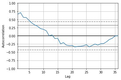
Below code plots, both ACF and PACF plots for us
from pandas.tools.plotting import autocorrelation_plot
from statsmodels.graphics.tsaplots import plot_pacf, plot_acf
autocorrelation_plot(df_log)
plot_pacf(df_log, lags=10)
plt.show()
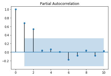
What suggests AR(q) terms in a model?
- ACF shows a decay
- PACF cuts off quickly
What suggests MA(p) terms in a model?
- ACF cuts off sharply
- PACF decays gradually
In PACF, the plot crosses the first dashed line(95% confidence interval line) around lag 4 hence p=4
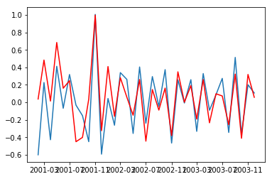
Below code fits an ARIMA model for us
from statsmodels.tsa.arima_model import ARIMA
model = ARIMA(df_log, order=(4,1,2))
result_AR = model.fit(disp=-1)
plt.plot(df_log_diff)
plt.plot(result_AR.fittedvalues, color='red')
plt.show()
Let us visualise the ARIMA model on shampoo prices.
Following code helps us to forecast shampoo sales for the next 4 months
future=df_log
future=future.reset_index()
mon=future["Date"]
mon=mon+pd.DateOffset(months=7)
future_dates = mon[-7-1:]
future = future.set_index('Date')
newDf = pd.DataFrame(index=future_dates, columns=future.columns)
future = pd.concat([future,newDf])
future["Forecast Sales"]= result_AR.predict(start=35, end =43, dynamic=True)
future["Forecast Sales"].iloc[-10:]=result_AR.forecast(steps=10)[0]
future[['Sales','Forecast Sales']].plot()
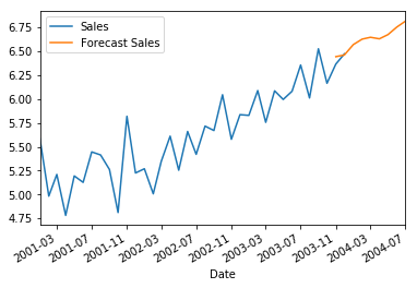
You can clearly see the predictions being made for the next 4 months!! Kudos to everyone for following till here.
Conclusion
Finally, we were able to build an ARIMA model and actually forecast for a future time period. Keep note that this is a basic implementation to get one started with time series forecasting. There are a lot of concepts like smoothening etc and models like ARIMAX, prophet etc to build your time series models. We will be covering more about time series in further blogs. Stay tuned!!
Follow this link, if you are looking to learn more about data science online!
You can follow this link for our Big Data course!
Additionally, if you are interested in learning Data Science, click here to get started
Furthermore, if you want to read more about data science, you can read our blogs here
Also, the following are some suggested blogs you may like to read

