Introduction
In computer science, Decision tree learning uses a decision tree (as a predictive model) to go from observations about an item to conclusions about the item’s target value. It is one of the predictive modelling approaches used in statistics, data mining and machine learning. Tree models where the target variable can take a discrete set of values are called classification trees and where the target variable can take continuous values (typically real numbers) are called regression trees.
In this blog, we will use decision trees to solve the churn problem for a telephonic service provider, Telco! The goal of this blog is about building a decision tree classifier. Furthermore, we will look at some metrics in the end in order to evaluate the performance of our decision tree model.
What is Customer Churn?
Churn is defined slightly differently by each organization or product. Generally, the customers who stop using a product or service for a given period of time are referred to as churners. As a result, churn is one of the most important elements in the Key Performance Indicator (KPI) of a product or service. A full customer lifecycle analysis requires taking a look at retention rates in order to better understand the health of the business or product.
From a machine learning perspective, churn can be formulated as a binary classification problem. Although there are other approaches to churn prediction (for example, survival analysis), the most common solution is to label “churners” over a specific period of time as one class and users who stay engaged with the product as the complementary class.
What is a Decision Tree?
Decision trees, one of the simplest and yet most useful Machine Learning structures. Decision trees, as the name implies, are trees of decisions.

You have a question, usually a yes or no (binary; 2 options) question with two branches (yes and no) leading out of the tree. You can get more options than 2, but for this article, we’re only using 2 options.
Trees are weird in computer science. Instead of growing from a root upwards, they grow downwards. Think of it as an upside down tree.
The top-most item, in this example, “Am I hungry?” is called the root. It’s where everything starts. Branches are what we call each line. A leaf is everything that isn’t the root or a branch.
Trees are important in machine learning as not only do they let us visualise an algorithm, but they are a type of machine learning.
Telco Customer Churn Problem Statement
Teleco is looking to predict behaviour to retain customers for their product. You can analyze all relevant customer data and develop focused customer retention programs.
Each row in the data represents a customer, each column contains customer’s attributes described in the column Metadata.
The data set includes information about:
- Customers who left within the last month — the column is called Churn
- Services that each customer has signed up for — phone, multiple lines, internet, online security, online backup, device protection, tech support, and streaming TV and movies
- Customer account information — how long they’ve been a customer, contract, payment method, paperless billing, monthly charges, and total charges
- Demographic info about customers — gender, age range, and if they have partners and dependents
You can access the data here!
Approach
1. Data Exploration
In this step, we will focus more on understanding data at hand. Before directly jumping to any modelling approach, one must understand the data at hand. We will look at different features/columns present in the data. We will also try to understand what every column relates too in the context of the Telco churn problem.
2. Data Preprocessing
There are very rare chances that data available at hand is directly applicable for building ML models. There can be multiple issues with data before you can even start implementing any fancy algorithm. Some of the issues can be missing values, improper format, the presence of categorical variables etc. We need to handle such issues then only we can train machine learning models. In our case of churn prediction, you can actually see our approach of handling missing data and categorical variables.
3. Training a decision tree classifier
In this section, we will fit a decision tree classifier on the available data. The classifier learns the underlying pattern present in the data and builds a rule-based decision tree for making predictions. In this section, we are focussing more on the implementation of the decision tree algorithm rather than the underlying math. But, we will cover some basic math behind it for your better understanding while implementing the decision tree algorithm. Also, you can read about the decision trees in detail here!
4. Model Evaluation
In this section, we will use our classifier to predict whether a customer will stop using the services of Telco or not. We will be looking at some of the methods like confusion matrix, AUC value and ROC-curve etc to evaluate the performance of our decision tree classifier.
Implementation in Python
We start by importing all the basic libraries and the data for training the decision tree algorithm. We are using numpy and pandas for performing mathematical operations and managing data in form of tables respectively.
import numpy as np # linear algebra
import pandas as pd # data processing, CSV file I/O (e.g. pd.read_csv)
import matplotlib.pyplot as plt # this is used for the plot the graph
import seaborn as sns # used for plot interactive graph.
import warnings
warnings.filterwarnings("ignore")
from pylab import rcParams
%matplotlib inline
data = pd.read_csv('./telco-churn.csv')
You can see the columns in the data below
######################### RESULT ###################################
<class 'pandas.core.frame.DataFrame'>
RangeIndex: 7043 entries, 0 to 7042
Data columns (total 21 columns):
customerID          7043 non-null object
gender              7043 non-null object
SeniorCitizen       7043 non-null int64
Partner             7043 non-null object
Dependents          7043 non-null object
tenure              7043 non-null int64
PhoneService        7043 non-null object
MultipleLines       7043 non-null object
InternetService     7043 non-null object
OnlineSecurity      7043 non-null object
OnlineBackup        7043 non-null object
DeviceProtection    7043 non-null object
TechSupport         7043 non-null object
StreamingTV         7043 non-null object
StreamingMovies     7043 non-null object
Contract            7043 non-null object
PaperlessBilling    7043 non-null object
PaymentMethod       7043 non-null object
MonthlyCharges      7043 non-null float64
TotalCharges        7043 non-null object
Churn               7043 non-null object
dtypes: float64(1), int64(2), object(18)
memory usage: 1.1+ MB
Customer ID contains no specific information about any customer hence we need to drop this column from our dataset
data=data.drop(['customerID'], axis=1)
Now, let us have a look at our target variable. Here the target variable is “Churn” i.e. if a customer is going to stop using the services of Telco or not. We can see the proportion of the people opting out of the Telco services (churners) through the following code. It builds a simple pie chart to show the distribution of two classes in the dataset.
# Data to plot for the % of target variable
labels =data['Churn'].value_counts(sort = True).index
sizes = data['Churn'].value_counts(sort = True)
colors = ["whitesmoke","red"]
explode = (0.1,0)  # explode 1st slice

rcParams['figure.figsize'] = 8,8
# Plot
plt.pie(sizes, explode=explode, labels=labels, colors=colors,
        autopct='%1.1f%%', shadow=True, startangle=270,)
plt.title('Percent of churn in customer')
plt.show()
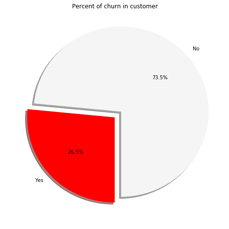
W can see through the pie chart, that 26.5% of customers present in the dataset are actually the churners i.e the people who opt out of the Telco services. The two target variables have a class imbalance in this case. No is present 73.5% of the times whereas yes is present only 26.5% of the times. In order to have a good machine learning model, we need to have a balance of the classes say 50% of both the class or in general, equal representation of the classes in the target variable.
There are techniques to manage the imbalanced classes like SMOTE but this is beyond the scope of this article for now. Decision trees can handle some imbalance present in the data better than other algorithms hence, we will not be using any technique to obtain balanced classes.
Finally, we need to convert yes/no of the target variable to 0 or 1. Machine learning models do not understand categorical variables. They need numbers to implement the underlying algorithms. Hence, our task in the data processing stage is to convert all the categorical variables to numbers.
# Converting the target class to 1’s and 0's
data['Churn'] = data['Churn'].map(lambda s :1  if s =='Yes' else 0)
Preprocessing Gender
In this section, we are processing the gender column to convert the categorical values into values. Pandas provide a get_dummies() function which can help you to convert your categorical column to a numeric one. It does one hot encoding of the values present in the column.
data['gender'].unique()
g = sns.factorplot(y="Churn",x="gender",data=data,kind="bar" ,palette = "Pastel1")
data = pd.get_dummies(data=data, columns=['gender'])
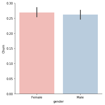
In this case, males and females have the same proportion of churning hence this variable is not informative enough to tell if a customer is going to stop using the services of Telco or not
Preprocessing Partner column
Partner columns contain a single yes/no. When there are only two categorical values present, we can directly replace the categories with 1 and 0. In case of more than two categorical variables, it is better to switch to one hot encoding of the values.
data['Partner'] = data['Partner'].map(lambda s :1 if s =='Yes' else 0)
Processing dependents, phone service and paperless billing variables
Above columns also contain only two categorical values. The following code assigns these categories a numeric 1/0 based on the respective category
data['Dependents'] = data['Dependents'].map(lambda s :1  if s =='Yes' else 0)
data['PhoneService'] = data['PhoneService'].map(lambda s :1  if s =='Yes' else 0)
data['PaperlessBilling'] = data['PaperlessBilling'].map(lambda s :1  if s =='Yes' else 0)
Analysing the number of months a person has stayed in the company
Let us analyse the number of months variable in order to understand the churn of the customers. We are plotting a distribution chart using the seaborn library in python through the following code!
# tenure distibution
g = sns.kdeplot(data.tenure[(data["Churn"] == 0) ], color="Red", shade = True)
g = sns.kdeplot(data.tenure[(data["Churn"] == 1) ], ax =g, color="Blue", shade= True)
g.set_xlabel("tenure")
g.set_ylabel("Frequency")
plt.title('Distribution of tenure comparing with churn feature')
g = g.legend(["Not Churn","Churn"])
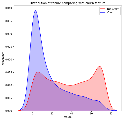
We can clearly observe that most numbers of customers leave before 20 months. Once a customer has stayed with Telco for more than 20 months, it is highly unlikely that he is going to stop using the services provided by the Telco
Handling the telephone lines variable
Converting telephone line variable into dummy values
data['MultipleLines'].replace('No phone service','No', inplace=True)
data['MultipleLines'] = data['MultipleLines'].map(lambda s :1  if s =='Yes' else 0)
Preprocessing Customer Service variable
Converting customer service variable into dummy values
data['Has_InternetService'] = data['InternetService'].map(lambda s :0  if s =='No' else 1)
data['Fiber_optic'] = data['InternetService'].map(lambda s :1  if s =='Fiber optic' else 0)
data['DSL'] = data['InternetService'].map(lambda s :1  if s =='DSL' else 0)
Preprocessing OnlineSecurity OnlineBackup DeviceProtection TechSupport StreamingTV StreamingMovie
data['OnlineSecurity'] = data['OnlineSecurity'].map(lambda s :1  if s =='Yes' else 0)
data['OnlineBackup'] = data['OnlineBackup'].map(lambda s :1  if s =='Yes' else 0)
data['DeviceProtection'] = data['DeviceProtection'].map(lambda s :1  if s =='Yes' else 0)
data['TechSupport'] = data['TechSupport'].map(lambda s :1  if s =='Yes' else 0)
data['StreamingTV'] = data['StreamingTV'].map(lambda s :1  if s =='Yes' else 0)
data['StreamingMovies'] = data['StreamingMovies'].map(lambda s :1  if s =='Yes' else 0)
Preprocessing payment and contract variables
data = pd.get_dummies(data=data, columns=['PaymentMethod'])
data = pd.get_dummies(data=data, columns=['Contract'])
Analysing monthly and total charges
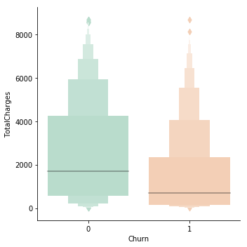
In this section, we will analyse the total and monthly charges column to understand their effect on the churning of the customers. Below code outputs a box plot based on the monthly charges between the customers who have left using the services and those who have not.
g = sns.factorplot(x="Churn", y = "MonthlyCharges",data = data, kind="box", palette = "Pastel1")
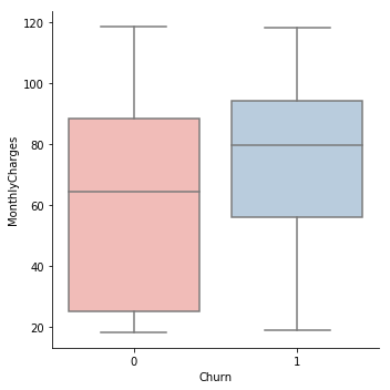
The high monthly charge is one cause for customers opting out of the services. The box plot also suggests that that loyal customers are those who have a low monthly charge.
data['TotalCharges'] = pd.to_numeric(data['TotalCharges'])
g = sns.factorplot(y="TotalCharges",x="Churn",data=data,kind="boxen", palette = "Pastel2")
Modeling
In this section, we are building our decision tree classifier. Decision tree algorithm has been implemented in the sklearn package and it provides an interface to invoke that algorithm.
We first separate out the target variables from the rest of our features present in the data. Following code performs this task
data["Churn"] = data["Churn"].astype(int)
Y_train = data["Churn"]
X_train = data.drop(labels = ["Churn"],axis = 1)
After that, we import the decision tree algorithm from the sklearn package. We pass the training data and the target data separately so that the algorithm can understand the input and create a rule-based mapping to the output in the form of a decision tree.
from sklearn import tree
# Initialize our decision tree object
classification_tree = tree.DecisionTreeClassifier(max_depth=4)
# Train our decision tree (tree induction + pruning)
classification_tree = classification_tree.fit(X_train, Y_train)
We can also visualise the trained decision tree in the previous step using the below code. Branches represent the actions while the internal nodes represent a decision. Leaf nodes represent the final target variables i.e whether a customer is churning or not (1/0)
import graphviz
dot_data = tree.export_graphviz(classification_tree, out_file=None,
                     feature_names=X_train.columns,
                     class_names="Churn",
                     filled=True, rounded=True,
                     special_characters=True)
graph = graphviz.Source(dot_data)
graph.render("data")
Before we move on to the evaluation of our algorithm, let us quickly test the accuracy of our model by making some predictions. Below code makes some predictions on the test data. We are using cross-validation here in order to avoid bias while testing the model for accuracy.
from sklearn.model_selection import  cross_val_score
# 10 Folds Cross Validation
clf_score = cross_val_score(classification_tree, X_train, Y_train, cv=10)
print(clf_score)
clf_score.mean()
##### RESULT #####################################################
[ 0.79403409  0.80397727  0.77698864  0.78805121  0.77809388  0.76671408
  0.80654339  0.78236131  0.78662873  0.8034188 ]
0.78868114065482486
Feature Importance
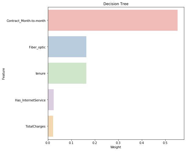
One great aspect of rule-based learning is that we can actually visualise how important a given feature is towards predicting our target variable. Below code forms a chart showing the relative importance of the features present in the data towards the prediction of our target churn class.
Rfclf_fea = pd.DataFrame(classification_tree.feature_importances_)
Rfclf_fea["Feature"] = list(X_train)
Rfclf_fea.sort_values(by=0, ascending=False).head()
g = sns.barplot(0,"Feature",data = Rfclf_fea.sort_values(by=0, ascending=False)[0:5], palette="Pastel1",orient = "h")
g.set_xlabel("Weight")
g = g.set_title("Decision Tree")
Evaluation
In order to evaluate our classification model, we are using the confusion matrix. A confusion matrix is a table that is often used to describe the performance of a classification model (or “classifier”) on a set of test data for which the true values are known.
You can read more about the confusion matrix here.
# Confusion Matrix
from sklearn.metrics import confusion_matrix
from sklearn.metrics import roc_auc_score
y_pred = classification_tree.predict(X_train)
probs = classification_tree.predict_proba(X_train)
print(confusion_matrix(Y_train, y_pred))
# calculate AUC
auc = roc_auc_score(Y_train, probs[:,1])
print('AUC: %.3f' % auc)
print(Y_train.shape)
print(probs.shape)
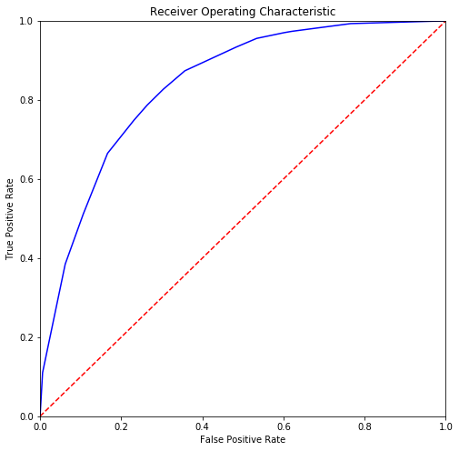
Following code generates the ROC curve for the predictions performed by our decision tree classifier. More the area under the ROC curve, better the prediction capability of the decision tree classifier.
from sklearn.metrics import roc_curve
# Calculate the fpr and tpr for all thresholds of the classification
fpr, tpr, threshold = roc_curve(Y_train, probs[:,1])
plt.title('Receiver Operating Characteristic')
plt.plot(fpr, tpr, 'b')
plt.plot([0, 1], [0, 1],'r--')
plt.xlim([0, 1])
plt.ylim([0, 1])
plt.ylabel('True Positive Rate')
plt.xlabel('False Positive Rate')
plt.show()
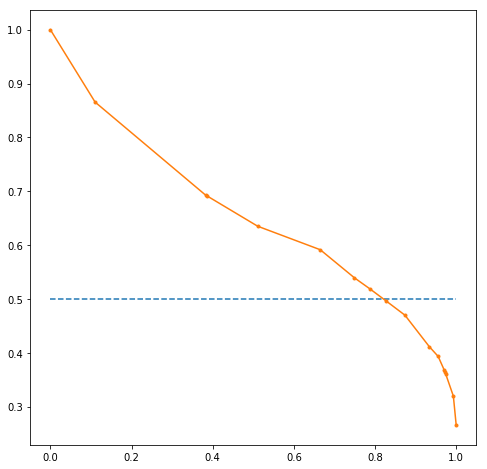
Below code makes a precision vs recall curve on the basis of the predictions. A precision-recall curve is a better indicator of the model performance than the ROC curve in case of imbalance in the target variable.
from matplotlib import pyplot
from sklearn.metrics import precision_recall_curve
precision, recall, thresholds = precision_recall_curve(Y_train, probs[:,1])
# plot no skill
pyplot.plot([0, 1], [0.5, 0.5], linestyle='--')
# plot the roc curve for the model
pyplot.plot(recall, precision, marker='.')
Summary
In this blog, we covered building a decision tree classifier for a sample use case. Decision trees can be a great platform to plant your footsteps in the world of machine learning as they are easier to implement and interpret. Also, we made some predictions using our decision tree classifier and evaluated its performance. The scope of this article was to familiarise the readers with decision trees and it’s an implementation for a use case!
For the next steps, you can also look at the Random Forest algorithm, which is nothing but a collection of different decision trees together making predictions. You can read more about the random forest here.
Follow this link, if you are looking to learn more about data science online!
You can follow this link for our Big Data course!
Additionally, if you are interested in learning Data Science, click here to get started
Furthermore, if you want to read more about data science, you can read our blogs here
Also, the following are some suggested blogs you may like to read

