Principal Component Analysis in R – Walk Through

Principal Component Analysis or PCA is one of the simplest and fundamental techniques used in machine learning. It is perhaps one of the oldest techniques available for dimensionality reduction, and thus, its understanding is of paramount importance for any aspiring Data Scientist/Analyst. An in-depth understanding of PCA in R will not only help in the implementation of effective dimensionality reduction but also help to build the foundation for development and understanding of other advanced and modern techniques.

PCA aims to achieve two primary goals:

1. Dimensionality Reduction

Real-life data has several features generated from numerous resources. However, our machine learning algorithms are not adept enough to handle high dimensions efficiently. Feeding several features, all at once, almost always leads to poor results since the models cannot grasp and learn from such volume altogether. This is called the “Curse of Dimensionality” which leads to unsatisfactory results from the models implemented. Principal Component Analysis in R helps resolve this problem by projecting n dimensions to n-x dimensions (where x is a positive number), preserving as much variance as possible. In other words, PCA in R reduces the number of features by transforming the features into a lesser number of projections of themselves.

2. Visualization

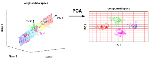
Our visualization systems are limited to 2-dimensional space which prevents us from forming a visual idea of the high dimensional features in the dataset. PCA in R resolves this problem by projecting n dimensions to a 2-D environment, enabling sound visualization. These visualizations sometimes reveal a great deal about the data. For instance, the new feature projections may form clusters in the 2-D space which was previously not perceivable in higher dimensions.

Intuition

Principal Component Analysis in R works with the simple idea of projection of a higher space to a lower space or dimension

The two alternate objectives of Principal Component Analysis are:

1. Variance Maximization Formulation

2. Distance Minimization Formulation

Let us demonstrate the above with the help of simple examples. If you have 2 features, and you wish to reduce the features to a 1-D feature set using PCA in R, you must lookout for the direction with maximal spread/variance. This becomes the new direction on which every data point is projected. The direction perpendicular to this direction has the least variance, and is thus, discarded.

Alternately, if one focuses on the perpendicular distance between a data point and the direction of maximum variance, our objective shifts to the minimization of that distance. This is because, lesser the distance, higher is the authenticity of the projection.

On completion of these projections, you would have successfully transformed your 2-D data to a 1-D dataset.

Mathematical Intuition

Principal Component Analysis in R locates the distance of maximal spread (or direction of minimal distance from data points) with the use of Eigen Vectors and Eigen Values. Every Eigen Vector (V_i) corresponds to an Eigen Value (E_i).

If X is a feature matrix (matrix with the feature values),

covariance matrix S = X^T. X

If E_iV_i = SV_{i ,}

Then Ei is an Eigen Value, and V_i becomes the corresponding Vector.

If there are d dimensions, there will be d Eigenvalues with d corresponding Eigen Vectors, such that:

E1>=E2>=E3>=E4>=…>=Ed

Each corresponding to V1, V2, V3, …., Vd

Here the vector corresponding to the largest Eigenvalue is the direction of Maximal spread since rotation occurs such that V1 is aligned with maximal variance in the feature space. Vd here has the least variance in its direction.

A very interesting property of Eigenvectors is the fact that if any two vectors are picked randomly from the set of d vectors, they will turn out to be perpendicular to each other. This happens because they align themselves such that they catch the most opposing directions in terms of variance.

When deciding between two Eigen Vector directions, Eigenvalues come into play. If V1 and V2 are two Eigen Vectors (perpendicular to each other), the values associated with these vectors, E1 and E2, help us identify the “percentage of variance explained” in either direction.

Percentage of variance explained Ei/(Sum(d Eigen Values)) where i is the direction we wish to calculate the percentage of variance explained for.

Implementation

Principal Component Analysis in R can either be applied with manual code using the above mathematical intuition, or it can be done using R’s inbuilt functions.

Even if the mathematical concept failed to leave a lasting impression on your mind, be assured that it is not of great consequence. On the other hand, understanding the basic high-level intuition counts. Without using the mathematical formulas, PCA in R can be easily applied using R’s prcomp() and princomp() functions which can be found here.

In order to demonstrate Principal Component Analysis, we will be using R, one of the most widely used languages in Data Science and Machine Learning. R was initially developed as a tool to aid researchers and scientists dealing with statistical problems in the academic field. With time, as more individuals from the academic spheres started seeping into the corporate and industrial sectors, they brought along R and its phenomenal uses along with them. As R got integrated into the IT sector, its popularity increased manifold and several revisions were made with the release of every new version. Today R has several packages and integrated libraries which enables developers and data scientists to instantly access statistical solutions without having to go into the complicated details of the operations. Principal Component Analysis is one such statistical approach which has been taken care of very well by R and its libraries.

For demonstrating PCA in R, we will be using the Breast Cancer Wisconsin Dataset which can be downloaded from here: Data Link

wdbc <- read.csv(“wdbc.csv”, header = F)

features <- c(“radius”, “texture”, “perimeter”, “area”, “smoothness”, “compactness”, “concavity”, “concave_points”, “symmetry”, “fractal_dimension”)

names(wdbc) <- c(“id“, “diagnosis“, paste0(features,”_mean“), paste0(features,”_se“), paste0(features,”_worst“))

These code statements help to read data into the variables wdbc.

wdbc.pr <- prcomp(wdbc[c(3:32)], center = TRUE, scale = TRUE)
summary(wdbc.pr)

The prcomp() function helps to apply PCA in R on the data variable wdbc. This function of R makes the entire process of implementing PCA as simple as writing just one line of code. The internal operations and functions are taken care of and are even optimized in terms of memory and performance to carry out the operations optimally. The range 3:32 is used to tell the function to apply PCA only on the features or columns which lie in the range of 3 to 32. This excludes the sample ID and diagnosis variables since they are identification columns and are invalid as features with no direct significance with regard to the target variable.

wdbc.pr now stores the values of the principal components.

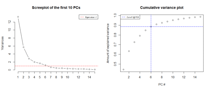
Let us now visualize the different attributes of the resulting Principal Components for the 30 features:

screeplot(wdbc.pr, type = "l", npcs = 15, main = "Screeplot of the first 10 PCs")

abline(h = 1, col="red", lty=5)

legend("topright", legend=c("Eigenvalue = 1"),
        col=c("red"), lty=5, cex=0.6)cumpro <- cumsum(wdbc.pr$sdev^2 / sum(wdbc.pr$sdev^2))

plot(cumpro[0:15], xlab = "PC #", ylab = "Amount of explained variance", main = "Cumulative variance plot")

abline(v = 6, col="blue", lty=5)

abline(h = 0.88759, col="blue", lty=5)

legend("topleft", legend=c("Cut-off @ PC6"),

       col=c("blue"), lty=5, cex=0.6)

This piece of code yields the following results:

Image Courtesy: towards data science

This plot clearly demonstrates that the first 6 components account for 90% of the variance in the dataset (with Eigen Value > 1). This means that one can easily exclude 24 features out of 30 features in order to preserve 90% of the data.

Limitations of PCA

Even though Principal Component Analysis in R displays a highly intuitive technique, it hosts certain shocking limitations.

1. Loss of Variance: If the percentage of variance against the chosen axis is around 50-60%, it is evident that 40-50% of the information which contributes to the variance of the dataset is lost during dimensionality reduction. This happens often when the data is spherical or bulging in nature.

2. Loss of Clusters: If there are several clusters present in the original dataset, but most of them lie in the direction perpendicular to the chosen direction. Thus, all the points from different clusters will be projected to the same region on the line of chosen direction, leading to one cluster of data points which are in fact quite different in nature.

3. Loss of Data Patterns: If the dataset forms a nice wavy pattern in direction of maximal spread, PCA takes to project all the points on the line aligned against the direction. Thus, data points which formed a wave function are concentrated on one-dimensional space.

These demonstrate how PCA in R, even though very effective for certain datasets, is a weak instrument for dimensionality reduction or visualization. To resolve these limitations to a certain extent, t-SNE, which is another dimensionality reduction algorithm, is used. Stay tuned to our blogs for a similar and well-guided walkthrough in t-SNE.

Follow this link, if you are looking to learn data science online!

You can follow this link for our Big Data course, which is a step further into advanced data analysis and processing!

Furthermore, if you want to read more about data science, read our Data Science Blogs