Modern technologies such as artificial intelligence, machine learning, data science, and Big Data have become the phrases everyone talks about, but no one fully understands them. To a layman, they seem very complex. All these words resemble a business executive or a student from a non-technical background. People are often confused by words such as AI, ML, and data science.
People are often confused about using technology for growing their business. With a plethora of technologies available and rise and shine of data science in recent times, the decision makes individuals & companies face the consent dilemma of whether to choose big data or ML or data science which can boost their businesses. In this blog, we will understand different concepts and have a look at this problem.
Let us understand key terms first i.e data science, machine learning, and big data
What is Data Science
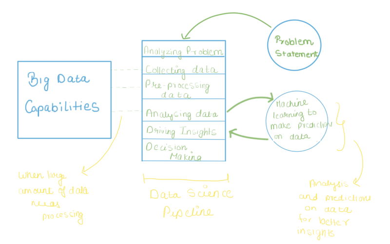
Data science is the umbrella under which all these terminologies take the shelter. Data science is a like a complete subject which has different stages within itself. Suppose a retailer wants to forecast the sales of an X item present in its inventory in the coming month. This is a business problem and data science aims to provide optimal solutions for the same.
Data science enables us to solve this business problem with a series of well-defined steps.
Collecting data
Pre-processing data
Analyzing data
Driving insights and generating BI report
Taking insight-bases decisions
Generally, these are the steps we mostly follow to solve a business problem. All the terminologies related to data science falls under different steps which we are going to understand just in a while. Different terminologies fall under different steps listed above.
You can learn more about the different component in data science from here
If you want to learn data science online then follow the link here
What is Big Data
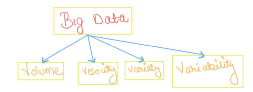
Big data is high-volume, high-velocity and/or high-variety information assets that demand cost-effective, innovative forms of information processing that enable enhanced insight, decision making, and process automation.
Characteristics Of ‘Big Data’
Volume — The name ‘Big Data’ itself is related to a size which is enormous. Size of data plays a very crucial role in determining value out of data. Also, whether a particular data can actually be considered as a Big Data or not, is dependent upon the volume of data. Hence, ‘Volume’ is one characteristic which needs to be considered while dealing with ‘Big Data’.
Variety — The next aspect of ‘Big Data’ is its variety. Variety refers to heterogeneous sources and the nature of data, both structured and unstructured. During earlier days, spreadsheets and databases were the only sources of data. Nowadays, analysis applications use data in the form of emails, photos, videos, monitoring devices, PDFs, audio, etc. This variety of unstructured-data poses certain issues for storage, mining and analyzing data.
Velocity — The term ‘velocity’ refers to the speed of generation of data. How fast the data is generated and processed to meet the demands, determines real potential in the data. Big Data Velocity deals with the speed at which data flows in from sources like business processes, application logs, networks, and social media sites, sensors, Mobile devices, etc. The flow of data is massive and continuous.
Variability — This refers to the inconsistency which can be shown by the data at times, thus hampering the process of being able to handle and manage the data effectively.
If you are looking to learn Big Data online then follow the link here
What is Machine Learning
At a very high level, machine learning is the process of teaching a computer system how to make accurate predictions when fed data.
Those predictions could be answering whether a piece of fruit in a photo is a banana or an apple, spotting people crossing the road in front of a self-driving car, whether the use of the word book in a sentence relates to a paperback or a hotel reservation, whether an email is a spam, or recognizing speech accurately enough to generate captions for a YouTube video.
The key difference from traditional computer software is that a human developer hasn’t written code that instructs the system how to tell the difference between the banana and the apple.
Instead, a machine-learning model has been taught how to reliably discriminate between the fruits by being trained on a large amount of data, in this instance likely a huge number of images labelled as containing a banana or an apple.
You can read more on how to be an expert in AI from here
The relationship between Data Science, Machine learning and Big Data
Data science is a complete journey of solving a problem using data at hand wheres Big data and machine learning are tools for the data scientists. It helps them to perform some specific tasks. While, Machine learning is more around making predictions using data present at hand whereas Big data emphasis on all the techniques that can be used to analyze a large set of data(thousands of petabytes may be, to begin with)
Let us understand in detail the difference between machine learning and Big Data
Big Data Analytics vs Machine Learning
You will find both similarities and differences when you compare between big data analytics and machine learning. However, the major differences lie in their application.
Big data analytics as the name suggest is the analysis of patterns or extraction of information from big data. So, in big data analytics, the analysis is done on big data. Machine learning, in simple terms, is teaching a machine how to respond to unknown inputs but still produce desirable outputs.
Most data analysis activities which do not involve expert task can be done through big data analytics without the involvement of machine learning. However, if the computational power required is beyond human expertise, then machine learning will be required.
Normal big data analytics is all about cleaning and transforming data to extract information, which then can be fed to a machine learning system in order to enable further analysis or predict outcomes without the requirement of human involvement.
Big data analytics and machine learning can go hand-in-hand and it would benefit a lot to learn both. Both fields offer good job opportunities as the demand is high for professionals across industries. When it comes to salary, both profiles enjoy similar packages. If you have skills in both of them, you are a hot property in the field of analytics.
However, if you do not have the time to learn both, you can go for whichever you are interested in.
So what to choose?
After understanding the 3 key phrases i.e Data science, Big data and machine learning, we are now in a better position to understand their selection and usage in business. We now know that data science is a complete process of using the power of data to boost business growth. So any decision-making process involving data has to involve data science.
There are few factors which may determine whether you should go for machine learning or Big data way for your organisation. Let us have a look at these factors and understand them in more detail
Factors affecting the selection
1. Goal
Selection of Big Data or Machine learning depends upon the end-goal of the business. If you are looking forward to generating predictions say based on customer behaviour or you want to build recommender systems then machine learning is the way to go. On the other hand, if you are looking for data handling and manipulation support where you can extract, load and transform data then Big Data will be the right choice for you.
2. Scale of operations
The scale of operation is one deciding factor between Big data and machine learning. If you have lots and lots of data like thousands of TB’s etc then employing Big data capabilities is the only choice. Traditional systems are not built to handle this much amount of data. Various businesses these days are sitting over huge chunks of data collected but lack the ability to meaningfully process them. Big Data systems allow handling of such amounts of data. Big data employs the concept of parallel computing which eases enables the systems to process and manipulate data in bulk quantities
3. Available resources
Employing Big data or machine learning capabilities requires a lot of investment both in terms of human resource and capital. If an organisation has resources trained for big data capabilities, then only they can manage such big infrastructure and leverage its benefits
Applications of Machine Learning
1. Image Recognition
It is one of the most common machine learning applications. There are many situations where you can classify the object as a digital image. For digital images, the measurements describe the outputs of each pixel in the image.
2. Speech Recognition
Speech recognition (SR) is the translation of spoken words into text. It is also known as “automatic speech recognition” (ASR), “computer speech recognition”, or “speech to text” (STT).
3. Learning Associations
Learning association is the process of developing insights into various associations between products. A good example is how seemingly unrelated products may reveal an association with one another. When analyzed in relation to buying behaviours of customers.
4. Recommendation systems
These applications have been the bread and butter for many companies. When we talk about recommendation systems, we are referring to the targeted advertising on your Facebook page, the recommended products to buy on Amazon, and even the recommended movies or shows to watch on Netflix.
Applications of Big Data
1. Government
Big data analytics has proven to be very useful in the government sector. Big data analysis played a large role in Barack Obama’s successful 2012 re-election campaign. The Indian Government utilizes numerous techniques to ascertain how the Indian electorate is responding to government action, as well as ideas for policy augmentation.
2. Social Media Analytics
The advent of social media has led to an outburst of big data. Various solutions have been built in order to analyze social media activity like IBM’s Cognos Consumer Insights, a point solution running on IBM’s BigInsights Big Data platform, can make sense of the chatter. Social media can provide valuable real-time insights into how the market is responding to products and campaigns. With the help of these insights, the companies can adjust their pricing, promotion, and campaign placements accordingly.
3. Technology
The technological applications of big data comprise of the following companies which deal with huge amounts of data every day and put them to use for business decisions as well. For example, eBay.com uses two data warehouses at 7.5 petabytes and 40PB as well as a 40PB Hadoop cluster for search, consumer recommendations, and merchandising. Inside eBay‟s 90PB data warehouse. Amazon.com handles millions of back-end operations every day, as well as queries from more than half a million third-party sellers.
4. Fraud detection
For businesses whose operations involve any type of claims or transaction processing, fraud detection is one of the most compelling Big Data application examples. Big Data platforms that can analyze claims and transactions in real time, identifying large-scale patterns across many transactions or detecting anomalous behaviour from an individual user, can change the fraud detection game.
Examples
1. Amazon
Amazon employs both machine learning and big data capabilities to serve its customers. It uses ML in form of recommender systems to suggest new products to its customers. They use big data to maintain and serve all the products data they have. Right from processing all the images and the content, to displaying them over the website, it is handled by the employed big data systems.
2. Facebook
Facebook similarly like Amazon has loads and loads of user data available with it. It uses machine learning to segment all the users based on their activity. Then, Facebook finds the best advertisements for its users in order to increase the clicks on the ads. All this is done through machine learning. With large user data at disposal, traditional systems can not process this data and make it ready for machine learning purposes. Facebook has employed big data systems so that they can process and transform this huge data and actually can derive insights out of it. Big data is required to make all this huge data processable.
Conclusion
In this blog, we learned how data science, machine learning and Big data link with each other. Whenever you want to solve any problem by using data at hand, data science is the process to solve it. If the data is too large and traditional systems or small-scale machines cannot handle it then BIG data techniques are the option to analyze such large chunks of data set. Machine learning covers the part when you want to make predictions of some kind, based on data you have at your end. These predictions will help you in validating your hypothesis around data and will enable smarter decision making.
Follow this link, if you are looking to learn more about data science online!
For those of you who don’t know, Julia is a multiple-paradigm (fullyimperative, partially functional, and partially object-oriented) programming language designed for scientific and technical (read numerical) computing. It offers significant performance gains over Python (when used without optimization and vectorized computing using Cython and NumPy). Time to develop is reduced by a factor of 2x on average. Performance gains range in the range from 10x-30x over Python (R is even slower, so we don’t include it. R was not built for speed). Industry reports in 2016 indicated that Julia was a language with high potential and possibly the chance of becoming the best option for data science if it received advocacy and adoption by the community. Well, two years on, the 1.0 version of Julia was out in August 2018 (version 1.0), and it has the advocacy of the programming community and the adoption by a number of companies (see https://www.juliacomputing.com) as the preferred language for many domains – including data science.
From https://blog.simos.info/learning-the-julia-computer-language-on-ubuntu/
While it shares many features with Python (and R) and various other programming languages like Go and Ruby, there are some primary factors that set Julia apart from the rest of the competition:
Advantages of Julia
Performance
Basically, Julia is a compiled language, whereas Python and R are interpreted. That means that Julia code is executed directly on the processor as executable code. There are optimizations that can be done for compiler output that cannot be done with an interpreter. You could argue that Python, which is implemented in C as the Cython package, can be optimized to Julia-like levels of performance, can also be optimized if you know the language well. But the real answer to the performance question is that Julia gives you C-like speed without optimization and hand-crafted profiling techniques. If such performance is available without optimization in the first place, why go for Python? Juia could well be the solution to all your performance problems.
Having said that, Julia is still a teenager as far as growth and development maturity as a programming language is concerned. Certain operations like I/O cause the performance to drop rather sharply if not properly managed. From experience, I suggest that if you plan to implement projects in Julia, go for Jupyter Notebooks running Julia 1.0 as a kernel. The Juno IDE on the Atom editor is the recommended environment, but the lack of a debugger is a massive drawback if you want to use Julia code in production in a Visual Studio-like environment. Jupyter allows you to develop your code one feature at a time, and easy access to any variable and array values that you need to ‘watch’. The Julia ecosystem has an enthusiastic and broad community developing it, but since the update to 1.0 was less than six months ago, not all the packages in Julia from version 0.7 have been migrated completely, so you could come up with the odd package versioning problem while installing necessary packages for your project.
HPC Laptop use (from Unsplash)
2. GPU Support
This is directly related to performance. GPU support is handled transparently by some packages like TensorFlow.jl and MXNet.jl. For developers in 2018 already using extremely powerful GPUs for various applications with CUDA or cryptocurrency mining (just to take two common examples), this is a massive bonus, and performance boosts can even go anywhere between 100x to even 1000x for certain operations and configurations. If you want certain specific GPU capacity, Julia has you covered with libraries like cuBLAS.jl and cuDNN.jl for vendor-specific and CUDANative.jl for hand-crafted GPU programming and support. Low-level CUDA programming is also possible in Julia with CUDAdrv.jl and the runtime library CUDArt.jl. Clearly, Julia has evolved well beyond standard GPU support and capabilities. And even as you read this article, an active community is at work to extend and polish the GPU support for Julia.
3. Smooth Learning Curve, and Extensive Built-in Functionality
Julia is remarkably simple to learn and enjoyable to use. If you are a Python program, you will feel completely at home using Julia. In Julia, everything is an expression and there is basic functional programming support. Higher order functions are supported by simple assignment (=) and the function operator -> (lambda in Python, => in C#). Multidimensional matrix support is excellent – functions for BLAS and LINPACK packages are included in the LinearAlgebra package of the standard library. Rows are separated with the comma(,) delimiter, and columns with the semicolon(;) during initialization. Matrix transpose, adjoint, factorization, matrix division, identity, slicing, linear equation system solving, triangulization, and many more functionalities are single function callsaway. Even jagged multidimensional matrix support is available. Missing, nothing, any, all, isdef, istype, oftype, hash, Base as a parent class for every Julia object, isequal, and even undef (to represent uninitialized values) are just a few of the many keywords and functions available to increase the readability of your code. Other notable features include built-in support for arbitrary precision arithmetic, complex numbers, Dictionaries, Sets, BitStrings, BitArrays, and Pipelines. I have just scratched the surface here. The extensive built-in functionality is one of Julia’s best features, with many more easily available and well-documented modules.
4. Multiple Dispatch
This is a central core feature of the Julia programming language. Multiple dispatch or the multimethod functionality basically means that functions can be called dynamically at run-time to behave in different ways depending upon more than just the arguments passed (which is called function overloading) and can instead vary upon the objects being passed into it dynamically at runtime. This concept is fundamentally linked to the Strategy and Template design patterns in object-oriented terminology. We can vary the behaviour of the program depending upon any attribute as well as the calling object and the objects being passed into the function at runtime. This is one of the killer features of Julia as a language. It is possible to pass any object to a function and thus dynamically vary its behaviour depending upon any minute variation in its implementation, and in many cases, the standard library is built around this concept. Some research statistics indicate that the average lines of boilerplate code required in a complex system is reduced by a factor of three or more (!) by this language design choice. This simplifies development in highly complex software systems considerably and cleanly, without any unpredictable or erratic behaviour. It is, therefore, no surprise that Julia is receiving the acclaim now thatit richly deserves.
5. Distributed and Parallel Computing Support
Julia supports parallel and distributed computing using multiple topologies transparently. There is support for coroutines, like in the Go programming language, which are helper functions that operate in parallel on multicore architectures. There is extensive support for threads and synchronization primitives have been carefully designed to maximize performance and minimize the risk of race conditions. Through simple text macros and decorators/annotations like @Parallel, any programmer can write code that executes in parallel. OpenMP support is also present for executing parallel code with compiler directives and macros. From the beginning of its existence, Julia was a language designed to support high-performance computing with multiple worker processes executing simultaneously. And this makes it much easier to use for parallel computing than (say) Python, which has always had the GIL (Global Interpreter Lock for threads) as a serious performance problem.
6. Interoperation with other programming languages (C, Java, Python, etc)
Julia can call C, Go, Java, MATLAB, R, and Python code using native wrapper functions – in fact, every commonly used programming language today has interoperability support with Julia. This makes working with other languages infinitely easier. The only major difference is that in Julia, array indexes begin at 1 (like R) whereas in many other languages it begins at 0 (C, C++, Java, Python, C#, and many more). The interoperability support makes life as a Julia developer much simpler and easier than if you were working in Python or C++/Java. In the real world, calling other libraries and packages is a part of the data scientist’s daily routine – part of a developer’s daily routine. Open source packages are at an advantage here since they can be modified as required for your problem domain. Interoperability with all the major programming languages is one of Julia’s strongest selling points.
Programming Fundamentals 🙂
Current Weaknesses
Julia is still developing despite the 1.0 release. Performance, the big selling point, is affected badly by using global variables and the first run of a program is always slow, compared to execution following the first. The core developers of the Julia language need to work on its package management system, and critically, migration of all the third-party libraries to version 1.0. Since this is something that will happen over time with active community participation (kind of like the Python 2.7 to 3.6 migration, but with much less difficulty), this is an issue that will resolve itself as time goes by. Also, there needs to be more consistency in the language for performance on older devices. Legacy systems without quality GPUs could find difficulties in running Julia with just CPU processing power. (GPUs are not required, but are highly recommended to run Julia and for the developer to be optimally productive, especially for deep learning libraries likeKnet (Julia library for neural networks and deeplearning)). The inclusion of support for Unicode 11.0 can be a surprise for those not accustomed to it, and string manipulation can be a headache. Because Julia needs to mature a little more as a language, you must also be sure to use aprofiler to identify and handle possible performance bottlenecks in your code.
Conclusion
So you might ask yourself a question – if you’re a company running courses in R and Python, why would you publish an article that advocates another language for data science? Simple. If you’re new to data science and programming, learning Python and R is the best way to begin your exploration into the current industry immediately (it’s rather like learning C before C++). And Python and R are not going anywhere anytime soon. Since there is both a massive codebase and a ton of existing frameworks and production code that run on Python and to a lesser level, on R, the demand for data scientists who are skilled in Python will extend far into the future. So yes, it is fully worth your time to learn both Python and R. Furthermore, Julia has yet to be adopted industry-wide (although there are many Julia evangelists who promote it actively – e.g. see www.stochasticlifestyle.com). For at least ten years more, expect Python to be the main player as far as data science is concerned.
Furthermore, programming languages never fully die out. COBOL wasdesigned by a committee led by Grace Hopper in 1959 and is still the go-to language for mainframe programming fifty years later. Considering that, expect the ubiquitously used Python and R to be market forces for at least two decades more. Even if more than 70% of the data science community turned to Julia as the first choice for data science, the existing codebase in Python and R will not disappear any time soon. Julia also requires more maturity as a language (as already mentioned) – some functions run slower than Python where the implementation has not been optimal and well tested, especially on older devices. Hence, Julia’s maturity as a programming language could still be a year or two away. So – reading this article, realize that Python and R are very much prerequisite skills in becoming a professional data scientist right now. But – do explore Julia a little in your free time. All the best!
For further information on choosing data science as a career, I highly recommend the following articles:
The constant evolution of technology has meant data and information is being generated at a rate unlike ever before, and it’s only on the rise. Furthermore, the demand for people skilled in analyzing, interpreting and using this data is already high and is set to grow exponentially over the coming years. These new roles cover all aspect from strategy, operations to governance. Hence, the current and future demand will require more data scientists, data engineers, data strategists, and Chief Data Officers.
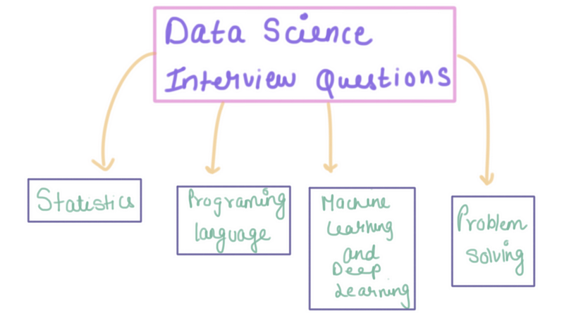
In this blog, we will be looking at different set of interview questions that can certainly help if you are planning to give a shift to your career towards data science.
Category of Interview Questions
Statistics
1. Name and explain few methods/techniques used in Statistics for analyzing the data?
Answer:
Arithmetic Mean: It is an important technique in statistics Arithmetic Mean can also be called an average. It is the number or the quantity obtained by summing two or more numbers/variables and then dividing the sum by the number of numbers/variables.
Median:
Median is also a way of finding the average of a group of data points. It’s the middle number of a set of numbers. There are two possibilities, the data points can be an odd number group or it can be en even number group.
If the group is odd, arrange the numbers in the group from smallest to largest. The median will be the one which is exactly sitting in the middle, with an equal number on either side of it. If the group is even, arrange the numbers in order and pick the two middle numbers and add them then divide by 2. It will be the median number of that set.
Mode: The mode is also one of the types for finding the average. A mode is a number, which occurs most frequently in a group of numbers. Some series might not have any mode; some might have two modes which is called bimodal series.
In the study of statistics, the three most common ‘averages’ in statistics are Mean, Median and Mode.
Standard Deviation (Sigma): Standard Deviation is a measure of how much your data is spread out in statistics.
Regression: Regression is an analysis in statistical modelling. It’s a statistical process for measuring the relationships among the variables; it determines the strength of the relationship between one variable and a series of other changing independent variables.
2. Explain about statistics branches?
Answer:
The two main branches of statistics are descriptive statistics and inferential statistics.
Descriptive statistics: Descriptive statistics summarizes the data from a sample using indexes such as mean or standard deviation.
Descriptive Statistics, methods include displaying, organizing and describing the data.
Inferential Statistics: Inferential Statistics draws the conclusions from data that are subject to random variation such as observation errors and sample variation.
3. List all the other models work with statistics to analyze the data?
Answer:
Statistics along with Data Analytics analyzes the data and help business to make good decisions. Predictive ‘Analytics’ and ‘Statistics’ are useful to analyze current data and historical data to make predictions about future events.
4. List the fields, where statistic can be used?
Answer:
Statistics can be used in many research fields. Below are the lists of files in which statistics can be used
Science
Technology
Business
Biology
Computer Science
Chemistry
It aids in decision making
Provides comparison
Explains action that has taken place
Predict the future outcome
Estimate of unknown quantities.
5. What is a linear regression in statistics?
Answer: Linear regression is one of the statistical techniques used in a predictive analysis, in this technique will identify the strength of the impact that the independent variables show on deepened variables.
6. What is a Sample in Statistics and list the sampling methods?
Answer:
In a Statistical study, a Sample is nothing but a set of or a portion of collected or processed data from a statistical population by a structured and defined procedure and the elements within the sample are known as a sample point.
Below are the 4 sampling methods:
Cluster Sampling: IN cluster sampling method the population will be divided into groups or clusters.
Simple Random: This sampling method simply follows the pure random division.
Stratified: In stratified sampling, the data will be divided into groups or strata.
Systematical: Systematical sampling method picks every kth member of the population.
7. What is P- value and explain it?
Answer:
When we execute a hypothesis test in statistics, a p-value helps us in determine the significance of our results. These Hypothesis tests are nothing but to test the validity of a claim that is made about a population. A null hypothesis is a situation when the hypothesis and the specified population is with no significant difference due to sampling or experimental error.
8. What is Data Science and what is the relationship between Data science and Statistics?
Answer: Data Science is simply data-driven science, also, it involves the interdisciplinary field of automated scientific methods, algorithms, systems, and process to extracts the insights and knowledge from data in any form, either structured or unstructured. Furthermore, It has similarities with data mining, both abstracts the useful information from data.
Data Sciences include Mathematical Statistics along with Computer science and Applications. Also by combing aspects of statistics, visualization, applied mathematics, computer science Data Science is turning the vast amount of data into insights and knowledge.
Similarly, Statistics is one of the main components of Data Science. Statistics is a branch of mathematics commerce with the collection, analysis, interpretation, organization, and presentation of data.
9. What is correlation and covariance in statistics?
Answer:
Covariance and Correlation are two mathematical concepts; these two approaches are widely used in statistics. Both Correlation and Covariance establish the relationship and also measure the dependency between two random variables. Though the work is similar between these two in mathematical terms, they are different from each other.
Correlation: Correlation is considered or described as the best technique for measuring and also for estimating the quantitative relationship between two variables. Correlation measures how strongly two variables are related.
Covariance: In covariance two items vary together and it’s a measure that indicates the extent to which two random variables change in cycle. It is a statistical term; it explains the systematic relation between a pair of random variables, wherein changes in one variable reciprocal by a corresponding change in another variable.
R is data analysis software which is used by analysts, quants, statisticians, data scientists, and others.
2. List out some of the function that R provides?
The function that R provides are
Mean
Median
Distribution
Covariance
Regression
Non-linear
Mixed Effects
GLM
GAM. etc.
3. Explain how you can start the R commander GUI?
Typing the command, (“Rcmdr”) into the R console starts the R Commander GUI.
4. In R how you can import Data?
You use R commander to import Data in R, and there are three ways through which you can enter data into it
You can enter data directly via Data New Data Set
Import data from a plain text (ASCII) or other files (SPSS, Minitab, etc.)
Read a dataset either by typing the name of the data set or selecting the data set in the dialogue box
5. Mention what does not ‘R’ language do?
Though R programming can easily connect to DBMS is not a database
R does not consist of any graphical user interface
Though it connects to Excel/Microsoft Office easily, R language does not provide any spreadsheet view of data
6. Explain how R commands are written?
In R, anywhere in the program, you have to preface the line of code with a #sign, for example
# subtraction
# division
# note order of operations exists
7. How can you save your data in R?
To save data in R, there are many ways, but the easiest way of doing this is
Go to Data > Active Data Set > Export Active dataset and a dialogue box will appear, when you click ok the dialogue box lets you save your data in the usual way.
8. Mention how you can produce co-relations and covariances?
You can produce co-relations by the cor () function to produce co-relations and cov() function to produce covariances.
9. Explain what is t-tests in R?
In R, the t.test () function produces a variety of t-tests. The t-test is the most common test in statistics and used to determine whether the means of two groups are equal to each other.
10. Explain what is With () and By () function in R is used for?
With() function is similar to DATA in SAS, it applies an expression to a dataset.
BY() function applies a function to each level of factors. It is similar to BY processing in SAS.
11. What are the data structures in R that are used to perform statistical analyses and create graphs?
In R missing values are represented by NA (Not Available), why impossible values are represented by the symbol NaN (not a number).
14. Explain what is transpose?
For re-shaping data before, analysis R provides a various method and transpose are the simplest methods of reshaping a dataset. To transpose a matrix or a data frame t () function is used.
15. Explain how data is aggregated in R?
By collapsing data in R by using one or more BY variables, it becomes easy. When using the aggregate() function the BY variable should be in the list.
Machine Learning
1. What do you understand by Machine Learning?
Answer:
Machine learning is an application of artificial intelligence that provides systems with the ability to automatically learn and improve from experience without being explicitly programmed. Also, machine learning focuses on the development of computer programs that can access data and use it learn for themselves.
2. Give an example that explains Machine Leaning in industry.
Answer:
Robots are replacing humans in many areas. It is because robots are programmed such that they can perform the task based on data they gather from sensors. They learn from the data and behaves intelligently.
3. What are the different Algorithm techniques in Machine Learning?
Answer:
The different types of Algorithm techniques in Machine Learning are as follows:
• Reinforcement Learning
• Supervised Learning
• Unsupervised Learning
• Semi-supervised Learning
• Transduction
• Learning to Learn
4. What is the difference between supervised and unsupervised machine learning?
Answer:
This is the basic Machine Learning Interview Questions asked in an interview. A Supervised learning is a process where it requires training labelled data While Unsupervised learning it doesn’t require data labelling.
5. What is the function of Unsupervised Learning?
Answer:
The function of Unsupervised Learning are as below:
• Find clusters of the data of the data
• Low-dimensional representations of the data
• Gaining interesting directions in data
• Interesting coordinates and correlations
• Figuring novel observations
6. What is the function of Supervised Learning?
Answer:
The function of Supervised Learning are as below:
• Classifications
• Speech recognition
• Regression
• Predict time series
• Annotate strings
7. What are the advantages of Naive Bayes?
Answer:
The advantages of Naive Bayes are:
• The classifier will converge quicker than discriminative models
• It cannot learn the interactions between features
8. What are the disadvantages of Naive Bayes?
Answer:
The disadvantages of Naive Bayes are:
• The problem arises for continuous features
• It makes a very strong assumption on the shape of your data distribution
• Does not work well in case of data scarcity
9. Why is naive Bayes so naive?
Answer:
Naive Bayes is so naive because it assumes that all of the features in a dataset are equally important and independent.
10. What is Overfitting in Machine Learning?
Answer:
This is the popular Machine Learning Interview Questions asked in an interview. Overfitting in Machine Learning is defined as when a statistical model describes random error or noise instead of underlying relationship or when a model is excessively complex.
11. What are the conditions when Overfitting happens?
Answer:
One of the important reason and possibility of overfitting is because the criteria used for training the model is not the same as the criteria used to judge the efficacy of a model.
12. How can you avoid overfitting?
Answer:
We can avoid overfitting by using:
• Lots of data
• Cross-validation
13. What are the five popular algorithms for Machine Learning?
Answer:
Below is the list of five popular algorithms of Machine Learning:
• Decision Trees
• Probabilistic networks
• Nearest Neighbor
• Support vector machines
• Neural Networks
14. What are the different use cases where machine learning algorithms can be used?
Answer:
The different use cases where machine learning algorithms can be used are as follows:
• Fraud Detection
• Face detection
• Natural language processing
• Market Segmentation
• Text Categorization
• Bioinformatics
15. What are parametric models and Non-Parametric models?
Answer:
Parametric models are those with a finite number of parameters and to predict new data, you only need to know the parameters of the model.
Non Parametric models are those with an unbounded number of parameters, allowing for more flexibility and to predict new data, you need to know the parameters of the model and the state of the data that has been observed.
16. What are the three stages to build the hypotheses or model in machine learning?
Answer:
This is the frequently asked Machine Learning Interview Questions in an interview. The three stages to build the hypotheses or model in machine learning are:
1. Model building
2. Model testing
3. Applying the model
17. What is Inductive Logic Programming in Machine Learning (ILP)?
Answer:
Inductive Logic Programming (ILP) is a subfield of machine learning which uses logical programming representing background knowledge and examples.
18. What is the difference between classification and regression?
Answer:
The difference between classification and regression are as follows:
• Classification is about identifying group membership while regression technique involves predicting a response.
• Both the techniques are related to prediction
• Classification predicts the belonging to a class whereas regression predicts the value from a continuous set
• Regression is not preferred when the results of the model need to return the belongingness of data points in a dataset with specific explicit categories
19. What is the difference between inductive machine learning and deductive machine learning?
Answer:
The difference between inductive machine learning and deductive machine learning are as follows:
machine learning where the model learns by examples from a set of observed instances to draw a generalized conclusion whereas in deductive learning the model first draws the conclusion and then the conclusion is drawn.
20. What are the advantages decision trees?
Answer:
The advantages decision trees are:
• Decision trees are easy to interpret
• Nonparametric
• There are relatively few parameters to tune
Answer:
The area of machine learning which focuses on deep artificial neural networks which are loosely inspired by brains. Alexey Grigorevich Ivakhnenko published the first general on working Deep Learning network. Today it has its application in various fields such as computer vision, speech recognition, natural language processing.
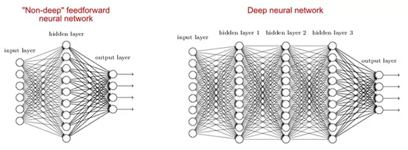
2. Why are deep networks better than shallow ones?
Answer:
There are studies which say that both shallow and deep networks can fit at any function, but as deep networks have several hidden layers often of different types so they are able to build or extract better features than shallow models with fewer parameters.
3. What is a cost function?
Answer:
A cost function is a measure of the accuracy of the neural network with respect to given training sample and expected output. It is a single value, nonvector as it gives the performance of the neural network as a whole. It can be calculated as below Mean Squared Error function:-
MSE=1n∑i=0n(Y^i–Yi)²
Where Y^ and desired value Y is what we want to minimize.
4. What is a gradient descent?
Answer:
Gradient descent is basically an optimization algorithm, which is used to learn the value of parameters that minimizes the cost function. Furthermore, It is an iterative algorithm which moves in the direction of steepest descent as defined by the negative of the gradient. We compute the gradient descent of the cost function for a given parameter and update the parameter by the below formula:-
Θ:=Θ–αd∂ΘJ(Θ)
Where Θ — is the parameter vector, α — learning rate, J(Θ) — is a cost function.
5. What is a backpropagation?
Answer:
Backpropagation is a training algorithm used for multilayer neural network. In this method, we move the error from an end of the network to all weights inside the network and thus allowing efficient computation of the gradient. It consists of several steps as follows:-
Forward propagation of training data in order to generate output.
Then using the target value and output value error derivative can be computed with respect to output activation.
Then we back propagate for computing derivative of error with respect to output activation on previous and continue this for all the hidden layers.
Using previously calculated derivatives for output and all hidden layers we calculate error derivatives with respect to weights.
And then we update the weights.
6. Explain the following three variants of gradient descent: batch, stochastic and mini-batch?
Answer:
Stochastic Gradient Descent: Here we use only single training example for calculation of gradient and update parameters.
Batch Gradient Descent: Here we calculate the gradient for the whole dataset and perform the update at each iteration.
Mini-batch Gradient Descent: It’s one of the most popular optimization algorithms. It’s a variant of Stochastic Gradient Descent and here instead of single training example, mini-batch of samples is used.
7. What are the benefits of mini-batch gradient descent?
Answer:
Below are the benefits of mini-batch gradient descent
•This is more efficient compared to stochastic gradient descent.
•The generalization by finding the flat minima.
•Mini-batches allows help to approximate the gradient of the entire training set which helps us to avoid local minima.
8. What is data normalization and why do we need it?
Answer:
Data normalization is used during backpropagation. The main motive behind data normalization is to reduce or eliminate data redundancy. Here we rescale values to fit into a specific range to achieve better convergence.
9. What is weight initialization in neural networks?
Answer:
Weight initialization is one of the very important steps. A bad weight initialization can prevent a network from learning but good weight initialization helps in giving a quicker convergence and a better overall error. Biases can be generally initialized to zero. The rule for setting the weights is to be close to zero without being too small.
10. What is an auto-encoder?
Answer:
An autoencoder is an autonomous Machine learning algorithm that uses backpropagation principle, where the target values are set to be equal to the inputs provided. Internally, it has a hidden layer that describes a code used to represent the input.
Some Key Facts about the autoencoder are as follows:-
•It is an unsupervised ML algorithm similar to Principal Component Analysis
•Minimizes the same objective function as Principal Component Analysis
•It is a neural network
•The neural network’s target output is its input
11. Is it OK to connect from a Layer 4 output back to a Layer 2 input?
Answer:
Yes, this can be done considering that layer 4 output is from previous time step like in RNN. Also, we need to assume that previous input batch is sometimes- correlated with the current batch.
12. What is a Boltzmann Machine?
Answer:
Boltzmann Machine is a method to optimize the solution of a problem. The work of the Boltzmann machine is basically to optimize the weights and the quantity for the given problem.
Some important points about Boltzmann Machine −
•It uses recurrent structure.
•Consists of stochastic neurons, which consist one of the two possible states, either 1 or 0.
•The neurons in this are either in adaptive (free state) or clamped (frozen state).
•If we apply simulated annealing on discrete Hopfield network, then it would become Boltzmann Machine.
13. What is the role of the activation function?
Answer:
The activation function is a method to introduce non-linearity into the neural network helping it to learn more complex function. Furthermore, without which the neural network would be only able to learn linear function which is a linear combination of its input data.
Follow this link if you are looking forward to becoming an AI expert
It is the perfect time to move ahead of the curve and position yourself with the skills needed to fill these emerging gaps in data science and analysis. Most importantly, this is not only for people who are at the very beginning of their careers and who decide on the path to study. Hence, professionals already in the workforce can benefit from this data science trend, perhaps even more than their fresh counterparts.
When I started my Data Science journey, I casually Googled ‘Application of Machine Learning Algorithms’. For the next 10 minutes, I had my jaw hanging. Quite literally. Part of the reason was that they were all around me. That music video from YouTube recommendations that you ended up playing hundred times on loop? That’s Machine Learning for you. Ever wondered how Google keyboard completes your sentence better than your bestie ever could? Machine Learning again!
So how does this magic happen? What do you need to perform this witchcraft? Before you move further, let me tell you who would benefit from this article.
Someone who has just begun her/his Data Science journey and is looking for theory and application on the same platter.
Someone who has a basic idea of probability and linear algebra.
Someone who wants a brief mathematical understanding of ML and not just a small talk like the one you did with your neighbour this morning.
Someone who aims at preparing for a Data Science job interview.
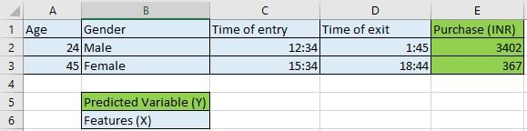
‘Machine Learning’ literally means that a machine (in this case an algorithm running on a computer) learns from the data it is fed. For example, you have customer data for a supermarket. The data consists of customers age, gender, time of entry and exit and the total purchase. You train a Machine Learning algorithm to learn the purchase pattern of customers and predict the purchase amount for a new customer by asking for his age, gender, time of entry and exit.
Now, Let’s dig deep and explore the workings of it.
Machine Learning (ML) Algorithms
Before we talk about the various classes, let us define some terms:
Seen data or Train Data –
This is all the information we have. For example, data of 1000 customers with their age, gender, time of entry and exit and their purchases.
Predicted Variable (or Y) –
The ML algorithm is trained to predict this variable. In our example, the ‘Purchase amount’. The predicted variable is usually called the dependent variable.
Features (or X) –
Everything in the data except for Y. Basically, the input that is fed to the model. Features are usually called the independent variable.
Model Parameters –
Parameters define our ML model. This will be understood later as we discuss each model. For now, remember that our main goal is to evaluate these parameters.
Unseen data or Test Data–
This is the data for which we have the X but not Y. The why has to be predicted using the ML model trained on the seen data.
Now that we have defined our terms, let’s move to the classes of Machine Learning or ML algorithms.
Supervised Learning Algorithms:
These algorithms require you to feed the data along with the predicted variable. The parameters of the model are then learned from this data in such a way that error in prediction is minimized. This will be more clear when individual algorithms are discussed.
Unsupervised Learning Algorithms:
These algorithms do not require data with predicted variables. Then what do we predict? Nothing. We just cluster these data points.
If you have any doubts about the things discussed above, keep on reading. It will get clearer as you see examples.
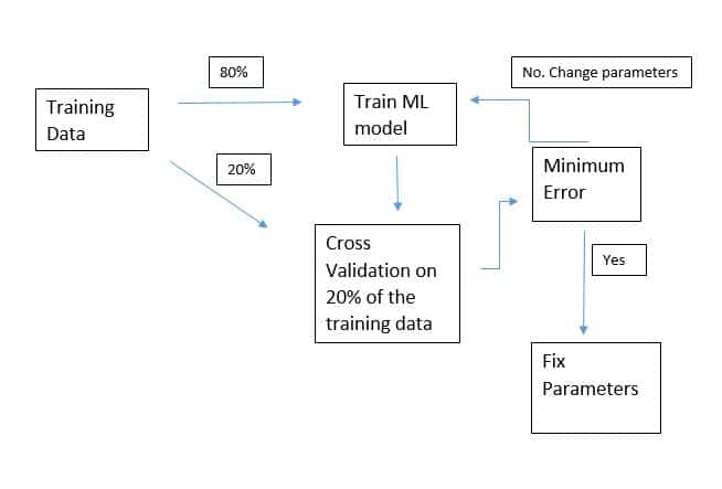
Cross-validation :
A general strategy used for setting parameters for any ML algorithm in general. You take out a small part of your training (seen) data, say 20%. You train an ML model on the 80% and then check it’s performance on that 20% of data (remember you have the Y values for this 20 %). You tweak the parameters until you get minimum error. Take a look at the flowchart below.
Supervised Learning Algorithms
In Supervised Machine Learning, there are two types of predictions – Regression or Classification. Classification means predicting classes of a data point. For example – Gender, Type of flower, Whether a person will pay his credit card bill or not. The predicted variable has 2 or more possible discrete values. Regression means predicting a numeric value of a data point. For example – Purchase amount, Age of a person, Price of a house, Amount of predicted rainfall, etc. The predicted class is a continuous variable. A few algorithms perform one of either task. Others can be used for both the tasks. I will mention the same for each algorithm we discuss. Let’s start with the most simple one and slowly move to more complex algorithms.
KNN: K-Nearest Neighbours
“You are the average of 5 people you surround yourself with”-John Rim
Congratulations! You just learned your first ML algorithm.
Don’t believe me? Let’s prove it!
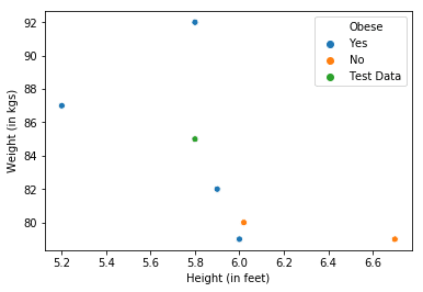
Consider the case of classification. Let’s set K, which is the number of closest neighbours to be considered equal to 3. We have 6 seen data points whose features are height and weight of individuals and predicted variable is whether or not they are obese.
Consider a point from the unseen data (in green). Our algorithm has to predict whether the person represented by the green data point is obese or not. If we consider it’s K(=3) nearest neighbours, we have 2 obese (blue) and one not obese (orange) data points. We take the majority vote of these 3 neighbours which is ‘Yes’. Hence, we predict this individual to be obese. In case of regression, everything remains the same, except that we take the average of the Y values of our K neighbours. How to set the value of K? Using cross-validation.
Key facts about KNN:
KNN performs poorly in higher dimensional data, i.e. data with too many features. (Curse of dimenstionality)
Euclidean distance is used for computing distance between continuous variables. If the data has categorical variables (gender, for example), Hamming distance is used for such variables. There are many popular distance measures used apart from these. You can find a detailed explanation here.
Linear Regression
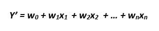
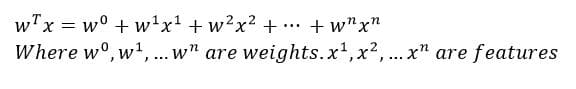
This is yet another simple, but an extremely powerful model. It is only used for regression purposes. It is represented by
….(1)
Y’ is the value of the predicted variable according to the model. X1, X2,…Xn are input features. Wo, W1..Wn are the parameters (also called weights) of the model. Our aim is to estimate the parameters from the training data to completely define the model.
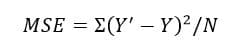
How do we do that? Let’s start with our objective which is to minimize the error in the prediction of our target variable. How do we define our error? The most common way is to use the MSE or Mean Squared Error –
For all N points, we sum the squares of the difference of the predicted value of Y by the model, i.e. Y’ and the actual value of the predicted variable for that point, i.e. Y.
We then replace Y’ with equation (1) and differentiate this MSE with respect to parameters W0,W1..Wn and equate it to 0 to get values of the parameters at which the error is minimum.
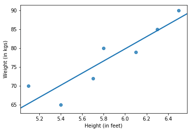
An example of how a linear regression might look like is shown below.
Sometimes it is not necessary that our dependent variable follows linear dependency on our independent variable. For example, Weight in the above graph may vary with the square of Height. This is called polynomial regression (Y varies with some power of X).
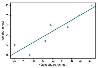
Good news is that any polynomial regression can be transformed to linear regression. How?
We transform the independent variable. Take a look at the Height variable in both the tables.
Table 1
table 2
We will forget about Table 1 and treat the polynomial regression problem like a linear regression problem. Only this time, Weight will be linear in Height squared (notice the x-axis in the figure below).
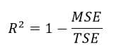
A very important question about every ML model one should ask is – How do you measure the performance of the model? One popular measure is R-squared
R-squared: Intuitively, it measures how well the data and hence the model explains the variation in the dependent variable. How? Consider the following question – If you had just the Y values and no X values in your data, and someone asks you, “Hey! For this X, what would you predict the Y to be?” What would be your best guess? The average of all the Y values you have! In this scenario of limited information, you are better off guessing the average of Y for any X than anything other value of Y.
But, now that you have X and Y values, you want to see how well your linear regression model predicts Y for any unseen X. R-squared quantifies the performance of your linear regression model over this ‘baseline model’
MSE is the mean squared error as discussed before. TSE is the total squared error or the baseline model error.
Naive Bayes
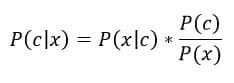
Naive Bayes is a classification algorithm. As the name suggests, it is based on Bayes rule.
Intuitive Breakdown of Bayes rule: Consider a classification problem where we are asked to predict the class of a data point x. We have two classes and the classes are denoted by letter C.
Now, P(c), also known as the ‘Prior Probability’ is the probability of a data point belonging to class C, when we don’t have any data. For example, if we have 100 roses and 200 sunflowers and someone asks you to classify an unseen flower while providing you with no information, what would you say?
P(rose) = 100/300 = ⅓ P(sunflower) = 200/300 = ⅔
Since P(sunflower) is higher, your best guess would be a sunflower. P(rose) and P(sunflower) are prior probabilities of the two classes.
Now, you have additional information about your 300 flowers. The information is related to thorns on their stem. Look at the table below.
Flower\Thorns
Thorns
No Thorns
Rose (Total 100)
90
10
Sunflower (Total 200)
50
150
Now come back to the unseen flower. You are told that this unseen flower has thorns. Let this information about thorns be X.
Now according to Bayes rule, the numerator for the two classes are as follows –
Rose = 1/3*9/10 = 3/10 = 0.3
Sunflower = 2/3*1/3 = 2/9 = 0.22
The denominator, P(x), called the evidence is the cumulative probability of seeing the data point itself. In this case it is equal to 0.3 + 0.22 = 0.52. Since it does not depend on the class, it won’t affect our decision-making process. We will ignore it for our purposes.
Since, 0.3>0.22
P(Rose|X) > P(sunflower|X)
Therefore, our prediction would be that the unseen flower is a Rose. Notice that our prior probabilities of both the classes favoured Sunflower. But as soon as we factored the data about thorns, our decision changed.
If you understood the above example, you have a fair idea of the Naive Bayes Algorithm.
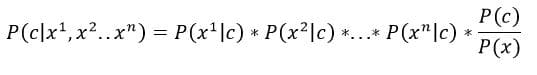
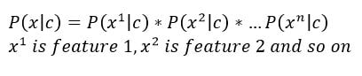
This simple example where we had only one feature (information about thorns) can be extended to multiple features. Let these features be x1, x2, x3 … xn. Bayes Rule would look like –
Note that we assume the features to be independent. Meaning,
The algorithm is called ‘Naive’ because of the above assumption
Logistic Regression
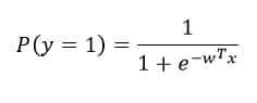
Logistic regression, unlike its name, is used for classification purposes. The mathematical model used for logistic regression is called the logit function. Consider two classes 0 and 1.
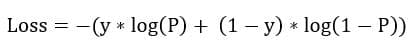
P(y=1) denotes the probability of belonging to class 1 and 1-P(y=1) is thus the probability of the data point belonging to class 0 (notice that the range of the function for all WT*X is between 0 and 1). Like other models, we need to learn the parameters w0, w1, w2, … wn to completely define the model. Like linear regression has MSE to quantify the loss for any error made in the prediction, logistic regression has the following loss function –
P is the probability of a data point belonging to class 1 as predicted by the model. Y is the actual class of the model.
Think about this – If the actual class of a data point is 1 and the model predicts P to be 1, we have 0 loss. This makes sense. On the other hand, if P was 0 for the same data point, the loss would be -infinity. This is the worst case scenario. This loss function is used in the Gradient Descent Algorithm to reach the parameters at which the loss is minimum.
Okay! So now we have a model that can predict the probability of an unseen data point belonging to class 1. But how do we make a decision for that point? Remember that our final goal is to assign classes, not just probabilities.
At what probability threshold do we say that the point belongs to class 1. Well, the model assigns the class according to the probabilities. If P>0.5, the class if obviously 1. However, we can change this threshold to maximize the metric of our interest ( precision, recall…), we can choose the best threshold using cross-validation.
This was Logistic Regression for you. Of course, do follow the coding tutorial!
Decision Tree
“Suppose there exist two explanations for an occurrence. In this case, the one that requires the least speculation is usually better.” – Occam’s Razor
The above philosophical principle precisely guides one of the most popular supervised ML algorithm. Decision trees, unlike other algorithms, are non-parametric algorithms. We don’t necessarily need to specify any parameter to completely define the model unlike KNN (where we need to specify K).
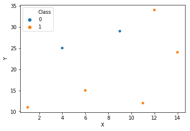
Let’s take an example to understand this algorithm. Consider a classification problem with two classes 1 and 0. The data has 2 features X and Y. The points are scattered on the X-Y plane as
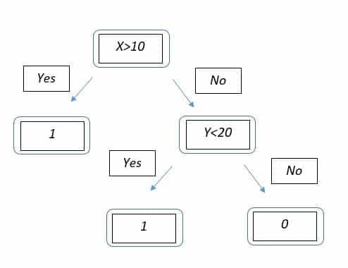
Our job is to make a tree that asks yes or no questions to a feature in order to create classification boundaries. Consider the tree below:
The tree has a ‘Root Node’ which is ‘X>10’. If yes, then the point lands at the leaf node with class 1. Else it goes to the other node where it is asked if its Y value is <20. Depending on the answer, it goes to either of the leaf nodes. Boundaries would look something like –
How to decide which feature should be chosen to bifurcate the data? The concept of ‘Purity ‘ is used here. Basically, we measure how pure (pure in 0s or pure in 1s) our data becomes on both the sides as compared to the node from where it was split. For example, if we have 50 1s and 50 0s at some node. After splitting, we have 40 1s and 10 0s on one side and 10 1s and 40 0s on the other, then we have a good splitting (one node is purer in 1s and the other in 0s). This goodness of splitting is quantified using the concept of Information Gain. Details can be found here.
Conclusion
If you have come so far, awesome job! You now have a fair level of understanding of basic ML algorithms along with their applications in Python. Now that you have a solid foundation, you can easily tackle advanced algorithms like Neural Nets, SVMs, XGBoost and many others.
The Nearest Neighbours algorithm is an optimization problem that was initially formulated in tech literature by Donald Knuth. The key behind the idea was to find out into which group of classes a random point in the search space belongs to, in a binary class, multiclass, continuous. unsupervised, or semi-supervised algorithm. Sounds mathematical? Let’s make it simple.
Imagine you are a shopkeeper who sells online. And you are trying to group your customers in such a way that products that are recommended for them come on the same page. Thus, a customer in India who buys a laptop will also buy a mouse, a mouse-pad, speakers, laptop sleeves, laptop bags, and so on. Thus you are trying to group this customer into a category. A class. How do you do this if you have millions of customers and over 100,000 products? Manual programming would not be the way to go. Here, the nearest neighbours method comes to the rescue.
You can group your customers into classes (for e.g. Laptop-Buyer, Gaming-Buyer, New-Mother, Children~10-years-old) and based upon what other people in those classes have bought in the past, you can choose to show them the items that they are the most likely to buy next, making their online shopping experience much easier and much more streamlined. How will you choose that? By grouping your customers into classes, and when a new customer comes, choosing which class he belongs to and showing him the products relevant for his class.
This is the essence of the ML algorithm that platforms such as Amazon and Flipkart use for every customer. Their algorithms are much more complex, but this is their essence.
The Nearest Neighbours topic can be divided into the following sub-topics:
Brute-Force Search
KD-Trees
Ball-Trees
K-Nearest Neighbours
Out of all of these, K-Nearest Neighbours (always referred to as KNNs) is by far the most commonly used.
K-Nearest Neighbours (KNNs)
A KNN algorithm is very simple, yet it can be used for some very complex applications and arcane dataset distributions. It can be used for binary classification, multi-class classification, regression, clustering, and even for creating new-algorithms that are state-of-the-art research techniques (e.g. https://www.hindawi.com/journals/aans/2010/597373/ – A Research Paper on a fusion of KNNs and SVMs). Here, we will describe an application of KNNs known as binary classification. On an extremely interesting dataset from the UCI-Repository (sonar.mines-vs-rocks).
Implementation
The algorithm of a KNN ML model is given below:
K-Nearest Neighbours
Again, mathematical! Let’s break it into small steps one at a time:
How the Algorithm Works
This explanation is for supervised learning binary classification.
Here we have two classes. We’ll call them A and B.
So the dataset is a collection of values which belong either to class A or class B.
A visual plot of the (arbitrary) data might look something like this:
Now, look at the star data point in the centre. To which class does it belong? A or B?
The answer? It varies according to the hyperparameters we use. In the above diagram, k is a hyperparameter.
They significantly affect the output of a machine learning (ML) algorithm when correctly tuned (set to the right values).
The algorithm then computes the ‘k’ points closest to the new point. The output is shown above when k = 3 and when k = 6 (k being the number of closest neighbouring points to indicate which class the new point belongs to).
Finally, we return a class as output which is closest to the new data point, according to various measures. The measures used include Euclidean distance among others.
This is how the K Nearest Neighbours algorithm works in principle. As you can see, visualizing the data is a big help to get an intuitive picture of what the k values should be.
Now, let’s see the K-Nearest-Neighbours Algorithm work in practice.
Note: This algorithm is powerful and highly versatile. It can be used for binary classification, multi-class classification, regression, clustering, and so on. Many use-cases are available for this algorithm which is quite simple but remarkably powerful, so make sure you learn it well so that you can use it in your projects.
Obtain the Data and Preprocess it
We shall use the data from the UCI Repository, available at the following link:
This data is a set of 207 sonar underwater readings by a submarine that have to be classified as rocks or underwater mines. Save the CSV file in the same directory as your Python source file and perform the following operations:
Import the required packages first:
import numpy as np
import pandas as pd
import scipy as sp


from datetime import datetime
from sklearn.preprocessing import LabelEncoder

from sklearn.model_selection import train_test_split
from sklearn.metrics.classification import accuracy_score
from sklearn.metrics.classification import confusion_matrix
from sklearn.metrics.classification import classification_report
Read the CSV dataset into your Python environment. And check out the top 5 rows using the head() Pandas DataFrame function.
Now, the last column is a letter. We need to encode it into a numerical value. For this, we can use LabelEncoder, as below:
#Inputs (data values) sonar readings from an underground submarine. Cool!
X = df.values[:,0:-1].astype(float)

# Convert classes M (Mine) and R to numbers, since they're categorical values
le = LabelEncoder()

#Classification target
target = df.R
# Do conversion
le = LabelEncoder.fit(le, y = ["R", "M"])
y = le.transform(target)
›
Now have a look at your target dataset. R (rock) and M (mine) has been converted into 1 and 0.
Execute the train_test_split partition function. This splits the inputs into 4 separate numpy arrays. We can control how the input data is split using the test_size or train_size parameters. Here the test size parameter is set to 0.3. Thus, 30% of the data goes into the test set and the remaining 70% (the complement) into the training set. We train (fit) the ML model on the training arrays and see how accurate our modes are on the test set. By default, the value is set to 0.25 (25%, 75%). Normally this sampling is randomized, so different results appear while being run each time. Setting random_state to a fixed value (any fixed value) makes sure that the same values are obtained every time we execute the model.
X_train, X_test, y_train, y_test = train_test_split(X, y, test_size=0.3, random_state=0)
Fit the KNN classifier to the dataset.
#Train kneighbors classifier
from sklearn.neighbors.classification import KNeighborsClassifier
clf = KNeighborsClassifier(n_neighbors = 5, metric = "minkowski", p = 1)

# Fit the model
clf.fit(X_train, y_train)
KNeighborsClassifier(algorithm='auto', leaf_size=30, metric='minkowski',
           metric_params=None, n_jobs=None, n_neighbors=5, p=1,
           weights='uniform')
As of now , it is all right (at this level) to leave the defaults as they are. The output of the KNeighborClassifier has two values that you do need to know: metric and p. Right now we just need the Manhattan Distance, specified by p = 1 and metric = “minkowski“, so we’ll go with that, which specifies Manhattan distance, which is, the distance between two points measured along axes at right angles. In a plane with p1 at (x1, y1) and p2 at (x2, y2), it is |x1 – x2| + |y1 – y2|. (Source: https://xlinux.nist.gov/dads/HTML/manhattanDistance.html)
Output the statistical scoring of this classification model.
Accuracy on the set was 82%. Not bad, since my first implementation was on random forests classifier and top score was just 72%!
The entire program as source code in Python is available here as a downloadable sonar-classification.txt file (rename *.txt to *.py and you’re good to go.):
K-Nearest-Neighbours is a powerful algorithm to have in your machine learning classification arsenal. It is used so frequently that most clustering models always start with KNNs first. Use it, learn it in depth, and it will be incredibly useful to you in your entire data science career. I highly recommend the Wikipedia article since it covers nearly all applications of KNNs and much more.
Finally, Understand the Power of Machine Learning
Imagine trying to create a classical reading of this sonar-reading with 60 features, trying to solve this reading from a non-machine learning environment. You would have to load a 207 X 61 ~ 12k samples. Then you would have to develop an algorithm by hand to analyze the data!
Scikit-Learn, TensorFlow, Keras, PyTorch, AutoKeras bring such fantastic abilities to computers with respect to problems that could not be solved in the past before ML came along.
And this is just the beginning!
Automation is the Future
As ML and AI applications take root in our world more and more, humanity will be replaced by ‘intelligent’ software programs that perform operations like a human. We have chatbots in many companies already. Self-driving cars daily push the very limits of what we think a machine can do. The only question is, will you be on the side that is being replaced or will you be on the new forefront of technological progress? Get reskilled. Or just, start learning! Today, as soon as you can.