source: medium
Data has consumed our day to day lives. The amount of data that’s is available in the web or from other variety of sources is more than enough to get an idea about any entity. The past few years has seen exponential rise in the volume which has resulted into the adaptation of the term Big Data. Most of these generated data are unstructured and could up in any format. Previously computers were not equipped to understand such unstructured data but modern computers coupled with some programs are able to mind such data and extract relevant information from it which has certainly helped many business.
Machine Learning is the study of predictive analytics where the structured or unstructured data are analysed and new results are predicted after the model is trained to learn the patterns from historical data. There are several pre-programmed Machine Learning algorithms which helps in building the model and the choice of the algorithm to be used completely depends on the problem statement, the architecture and the relationship among the variables.
However, the traditional state-of-the-art Machine Learning algorithms like Support Vector Machines, Logistic Regression, Random Forest, etc., often lacks efficiency when the size of the data increases. This problem is resolved by the advent of Deep Learning which is a sub-field of Machine Learning. The idea behind Deep Learning is more or less akin to our brain. The neural networks in Deep Learning works almost similarly to the neurons in the human brain.
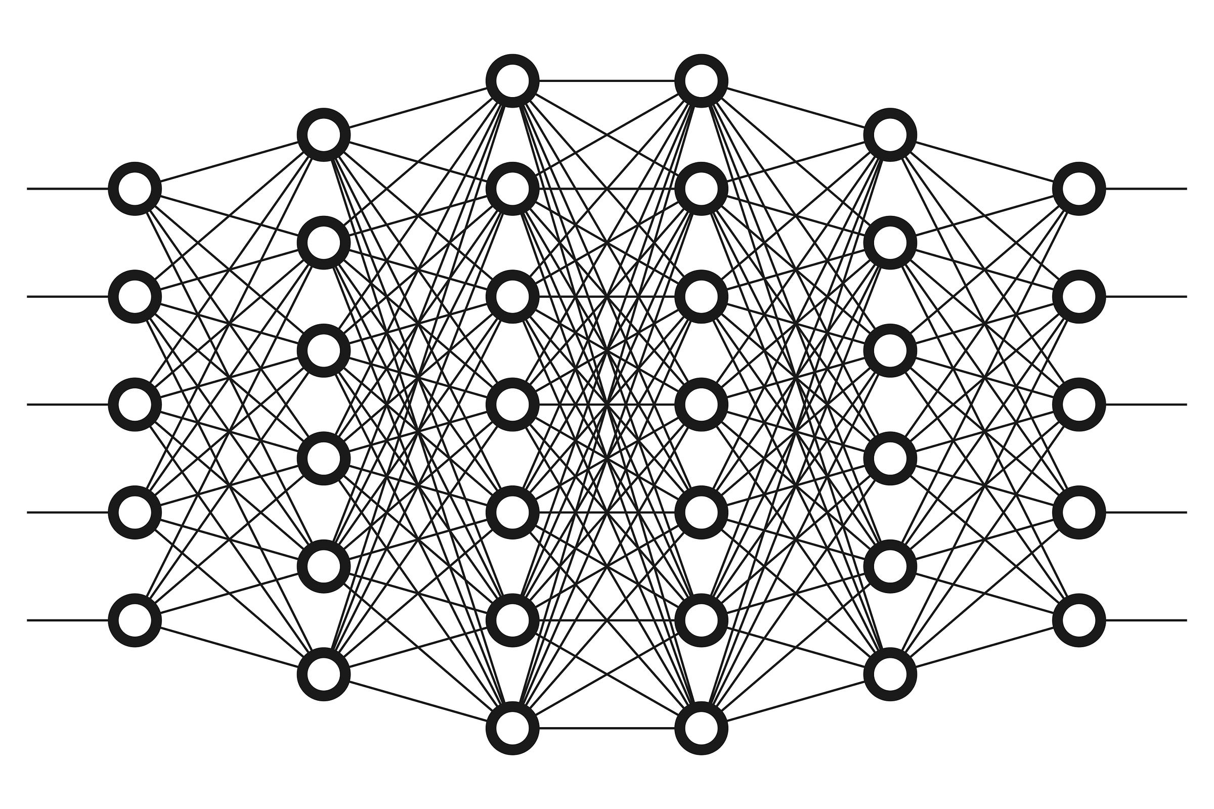
Deep Learning networks could be divided into Shallow Neural Networks and Deep L-Layered Neural Networks. In Shallow Neural Network, there is only one hidden layer along with the input and the output layers while in Deep L-Layered Neural Network there could be L number of small hidden layers along with the input and the output layers. On the contrary, computing some functions would require exponentially large shallow neural network and thus using a deep L-layered network is the best option in these scenarios. The choice of the activation function is Neural Network is an important step. In Binary classification problem, the sigmoid activation function is sufficient whereas in other problems, the Rectified Linear Unit activation function could be used. Some of the other important parameters in Deep Learning are Weights, Bias and hyper parameters such as the Learning rate, number of hidden layers, and so on.
To measure the performance of our Neural Network, one the best ways is to minimize the optimization function. For example – in Linear Regression, the optimization function is the Mean Squared Error and the lesser its value, the more accurate would be our model. In this blog post we would look into the optimization functions for Deep Learning.
Objective Functions in Deep Learning
To improve the performance of a Deep Learning model the goal is to the reduce the optimization function which could be divided based on the classification and the regression problems. Below are of some of objective functions used in Deep Learning.
1. Mean Absolute Error
In Regression problems, the intuition is to reduce the difference between the actual data points and the predicted regression line. Mean absolute error is one such function to do so which takes the mean of the absolute value of the difference between the actual and the predicted value for all the examples in the data set. The magnitude of errors are measured without the directions. Though it is a simple objective function but there is a lack of robustness and stability in this function. Also known as the L1 loss, its value ranges from 0 to infinity.
2. Mean Squared Error
Similar to the mean absolute error, instead of taking the absolute value, it squares the difference between the actual and the predicted data points. The squaring is done to highlight those points which are farther away from the regression line. Mean Squared Error is also known as the cost function in regression problems and the goal is to reduce the cost function to its global optimum in order to get the best fit line to the data.
This reduction in loss or the Gradient Descent is an incremental process where a value is initialized first and then the parameters are updated at each descent towards the global optimum. The speed of descent depends on the learning rate which needs to be adjusted as a very small value would lead to a slow step gradient descent while a larger value could fail to converge at all. Mean Squared Errors, however are sensitive to outliers. The range of values is always between 0 and infinity.
3. Huber
The penalty incurred by an estimation procedure f is described by the loss function Huber. For large values, the Huber function is linear while for small values, it is quadratic in nature. To make it quadratic, the magnitude by which the value needs to be small completely depends on the hyperparameter delta. This hyperparameter could be tuned as well.
Also known as the Smooth Mean Absolute Error, the sensitivity of Huber loss to outliers is less compared to the other functions. At zero, the Huber loss is differentiable. The Huber loss approaches Mean Absolute Error when the hyperparameter delta approaches to 0 and it approaches to the Mean Squared Error when the delta approaches to infinity. The value of delta would determine how much outlier you are willing to consider. L1 minimizes the residuals larger than delta while L2 minimizes the residuals smaller than delta.
4. Log-Cosh loss
A regression optimization function which is smoother than L2. The prediction error’s hyperbolic cosine’s logarithm is known as the log-cash loss function. For small value, it is equal to the half of its square while for large value, it equal to the difference between its absolute value of the logarithm of 2.
Log-cosh is not effected that much by occasional incorrect predictions and almost works similar to the mean squared error. Unlike Huber, it is twice differentiable. However, log-cosh often suffers from the Gradient problem.
5. Cosine Proximity
Between the predicted and the actual value, the cosine proximity is measured by this loss function which minimizes the dot product between them. There is maximal similarity between the unit vectors in this case if they are parallel which is represented by 0. However, in case of orthogonality, it is dissimilar represented by +1.
6. Poisson
The diversion of the predicted distribution from the expected distribution is measured by the Poisson loss function which is a Poisson distribution’s variant. For a normal approximation, the distribution is limited to a binomial as the probability becomes zero and trials becomes infinity. In Deep Learning, the Exponential Log Likelihood is similar to the Poisson.
7. Hinge
For training classifiers, the loss function which is used is known as the Hinge loss which follows the maximum-margin objective. The output of the predicted function in this case should be raw. The sign of the actual output data point and the predicted output would be same. The loss would be equal to zero when the predicted output is greater than 1. The loss increases linearly with the actual output data is the sign is not equal. In Support Vector Machines it is used mostly.
8. Cross Entropy
In Binary classification problem where the labels are either 0 or 1, the Cross Entropy loss function is used. The multiclass cross entropy however is used in case of multi-classification problem. Between two probability functions, the divergence is measured by the cross entropy function. Between two distributions, the difference would be large if the cross entropy is large but they are same when the difference is small. Cross entropy doesn’t suffer from the problem of slow divergence as seen in the mean squared error function due to the Sigmoid activation function.
The learning speed is fast when the difference is large and slow when the difference is small. Chances of reaching the global optimum is more in case of the cross entropy loss function because of its fast convergence.
9. Kullback-Leibler
The diversion of one probability distribution from a second expected probability distribution is measured by the Kullback-Leibler divergence also known as entropy, information divergence. Not considered as statistical measure of spread as it is a distribution wise asymmetric measure. Similarity is assumed when the value of Kullback-Leibler loss function is 0 while 1 indicates distributions behaving in a different manner.
10. Negative Logarithm Likelihood
Used widely in neural networks, the accuracy of a classifier is measured by the negative logarithm likelihood function. The idea of probabilistic confidence is followed by this function which outputs each class’s probability.
Conclusion
Deep Learning is one the growing fields in Data Science which thrives on more data. The concept of objective functions is crucial in Deep Learning as it needs to be optimized in order to get better prediction or a more efficient model.
Dimensionless has several blogs and training to get started with Python, and Data Science in general.
Follow this link, if you are looking to learn more about data science course online!
Additionally, if you are having an interest in learning Data Science, Learn online Data Science Course to boost your career in Data Science.
Furthermore, if you want to read more about data science, you can read our Data Science Blogs