Have you been lately flooded with different posts on your social media profiles showing people with their current age on the left and their older self on the right? If yes and If you are wondering how people are doing it, then I may have an answer to your query here. There is a new app (only available on ios for now), FaceApp, which is behind this rising trend on social media.
My initial guess was about that it must be one of the new image filter rolled out by Snapchat or Instagram but was clueless about the craze behind this trend. Since it’s similar to a 10-year challenge, rolled out by Facebook, earlier this year, there was no need for everyone to go crazy about this app. There are filters as well available which can make you look older. So why go bonkers over this new app?
If you look closely, results by FaceApp are much more realistic as compared to its image filter based counterparts in the Snapchat and Instagram. So what has FaceApp done which Snapchat and Instagram could not? We will try to answer this question in this blog. Before we proceed on to answer this question, let us understand what FaceApp is!
Courtesy: geekdashboard.com
What is FaceApp?
FaceApp is an IOS image processing app like many others on the app store which can process your images and bring changes to it. FaceApp was developed and released in 2016 by a small team of Russian developers. You can bring a selfie or use an ancient image from your phone and use a filter to use the app. The present free filters contain a smile that shows you old or young, sex bends, face hairs or the classic Walter White looks from the Breaking Bad TV series. The app gives its paying customers extra filters including maquilas, glasses and facial hair to their faces.
Changes include all the basic properties like contrast, brightness and sharpness to complex features like adding a smile, changing gender or showing an older/younger version of your self.
As previously said, all these features were available already on different apps as well but what makes the FaceApp really a winner is stark photo-realism. These images look more real and true rather than some blurry filter images. FaceApp with its surprisingly accurate image manipulation tricks has been able to gather a lot of attention because of which it has clocked over more than a million downloads in just 2 days. Rather than putting some creative or cartoonist filters over the images, FaceApp aims at manipulating the features present in the face in such a manner that it feels almost true to believe!
How is it different from Instagram filters?
So what is FaceApp doing differently? FaceApp rather than using image stacking or pixel manipulation uses Artificial Intelligence to bring the changes in the facial features. FaceApp makes use of the generative adversarial networks to create these images which are again too much realistic to be believed. Suppose you have a task of making a person smile in an image where he is not smiling at all. To make a person smile, extending the lips is not the only criteria. One needs to change all the facial features like eyes stretch, cheeks appearance in order to make the transformation realistic.
FaceApp has achieved this using GANs and this is exactly what is making this app stand out from the crowd. As far as we do not know of any other goods or studies of comparable performance in this field, FaceApp is far ahead in terms of the technology used. In the other section, let us dig deeper into the technique used by FaceApp
A Generative network is a type of AI machine learning (ML) method composed of two networks in a zero-sum game context that are in conflict with each other. GANs are usually unattended, teaching themselves how to imitate any specified information allocation.
There are two neural networks, the generator and the discriminator, that compose a GAN. The generator is a kind of neural system that creates fresh cases of an item, and the discriminator is a sort of neural network that determine its identity or whether it resides in a dataset.
During the teaching phase, both the models try to compete, their losses push each other towards improving behaviour and is called backpropagation. The generator’s objective is to generate reasonable performance while the discriminatory’s objective is to define the counterfeit. The generator generates high-quality results, and the discriminator is superior with the flagging components having a double feedback loop.
The first stage in the development of a GAN is for the required yield to be identified and the original learning data based on these parameters collect. This information are randomized and entered into the generator until the fundamental precision of the output is achieved.
Afterwards, the produced pictures and the real information points from the original concept are transmitted into the discriminator. The discriminator filters and gives the chance to reflect the validity of each image between 0 and 1 (1 corresponds to actual and 0 to falsify).
These values are then controlled manually and repeated until the required result is achieved. In a zero-sum game, both networks try to optimize a loss function.
Other use cases of GANs
Generating realistic photographs This use case revolves around generating new human faces which are too realistic that you won’t ever believe that there exists no person in the entire world with that face. Realism and use of state of the art artificial neural networks have made it possible to generate fake faces at ease. Realism in these images is the one key factor which has stirred the world and has made the use of GANs really attractive! You can view the example here which generated random faces using the generative adversarial networks
Image-to-Image Translation The image-to-image translation is the task of taking and transforming images from one domain to have the image style (or characteristics) from another.
Text-to-Image Translation In recent times, translation from text to the image has been an active field of research. A network’s capacity to understand the significance of a phrase and to create a precise picture depicting the phrase demonstrates a model’s capacity to more like people. Generative Adversarial Networks (GANs) are used to produce high-quality text input pictures through popular text to image translation techniques.
Proceed with caution
Experts have warned to allow them access to your personal details and identity by a FaceApp ancient age filter. FaceApp also involves in its terms and conditions, which you give the approval to access your picture gallery, the right of modifying, reproducing and publishing any image you process via its AI. This implies your face might finally be marketed.
By accepting the terms, we allow FaceApp to use, adapt, post, and distribute your user content in any media format on a perpetual, irrevocable, free of charge. This implies that you can use your actual name, your username or “any similarity is given” without notification, much less payment, in any format. You can keep it as long as you want and you can’t prevent it, even after you delete an app.
Summary
In this blog, we looked at the new emerging FaceApp which has gathered eyeballs all around. Furthermore, we also spent some time in understanding an overview of the technology which is behind this trending application. Although the faceApp has come with a breakthrough in the GANs technology and have set up high standards for the other apps, concerns around the data security and data-policy is still a concern with FaceApp.
You can follow this link for our Big Data course! This course will equip you with the exact skills required. Packed with content, this course teaches you all about AWS tools and prepares you for your next ‘Data Engineer’ role
Additionally, if you are having an interest in learning Data Science, click here to start the Online Data Science Course
Furthermore, if you want to read more about data science, read our Data Science Blogs
The flux of data is increasing exponentially in this age of Digital awakening. Data has become so important to major industries and sectors around the globe that it can literally be referred to as digital gold! From simple company centric applications to major platforms interweaving people from all around the world, data has started to shape major decisions for not only autonomous machines, but also for the human race as a whole. This imagery is as intriguing as it is terrifying, but only if we make it so.
In order to handle this rapidly incoming data with relative ease, a competent system is required to act instantly and deliver results on the fly. Otherwise, such large-scale investments on data gathering and data generation will go to waste since the data will be left in its dormant state without any active or competent agent acting on it. This is where the concept of real time data streaming and processing comes up. So, what is real time data streaming?
As is already known, data is being generated from various sources at a lightening pace. If we stop to ingest enough data, process it in batches and then provide the results after enough time has passed, the results will tend to lose its relevance and will reflect outdated patterns and trends. This happens majorly because of the high rate of variance in incoming data and also because of time constraints.
For instance, suppose that you have a machine which tells you which horse to bet upon in a horse race. You have the option of changing your choice during the race until the last lap commences. In such a case, if your machine gives you predictions based on the first lap where horse A was showing promise, and predicts that horse A will win, where in fact, during the third lap, horse B shows further promise, you will lose your bet just because of a machine which lags behind by two laps. This problem can be avoided by processing incoming data instantly, or in other words, real time data streaming. A stack of old data or historical data is studied and incoming records are processed based on the studied patterns such that the results are delivered within milliseconds. For our example, the horse race prediction machine would have already studied data about the different horses in the race previously and then based on the incoming data (the horse number, position of the horse, time since beginning of race, number of contestants, etc.), will be able to instantly allocate a rank for the different participants with the help of real time data streaming.
How to Go About Real-Time Data Streaming?
In real time mission-critical applications, Apache Kafka has turned out to be one of the most widely used frameworks for implementation. Apache Kafka is integrated with efficient machine learning frameworks in order to enable model training and speedy deliverance by supporting real time data streaming.
What is Apache Kafka?
As per Kafka’s website, it defines itself and its tasks as follows:
“Kafka® is used for building real-time data pipelines and streaming apps. It is horizontally scalable, fault-tolerant, wicked fast, and runs in production in thousands of companies.”
“The project aims to provide a unified, high-throughput, low-latency platform for handling real-time data feeds. Its storage layer is essentially a “massively scalable pub/sub message queue designed as a distributed transaction log”, making it highly valuable for enterprise infrastructures to process streaming data.” – Wikipedia
These definitions might seem like a mouthful at first, but as we go through with this subject step by step in this discussion, one will easily get the hang of it in no time!
Why use Tensorflow as the machine learning platform which is to be integrated with Apache Kafka?
Tensorflow is one of the most popular and efficient open source machine learning platforms available. It has a beautiful and well-suited architecture which enables data flow with extreme grace and optimization. It enables users and developers to establish large-scale projects with minimal hassles and maximal resource optimization. It is thus, a very competent platform to integrate with Apache Kafka for the purpose of serving real-time data streaming.
Tensorflow’s tf.keras and tf.data are responsible for streaming data in and out. Previously however, these modules were limited in their usage and could only support a few data formats. Support for Kafka streaming was not included during the earlier versions of Tensorflow. It was also difficult to use Tensorflow supported modules like tf. Examples and TFRecord in Big data and the general community of Data Science as a whole and were, therefore, rarely spotted.
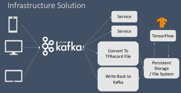
It was thus, a difficult task to integrate the Apache Kafka and Tensorflow frameworks. A lot of intermediary bridges had to be constructed in order to establish reliable handshakes between these two frameworks and ensure smooth integration. This was a burdensome process since it included designing of an entire infrastructure which turned out to be a fault prone mechanism most of the time. These were the steps which were required to be followed in order to establish a working data streaming flow:
Read data from the Kafka stream -> Convert to TFRecord format -> call Tensorflow’s function to read the TFRecord object from file system -> execute model and deliver result -> save the result in the file system again -> write results/ inference back to Kafka
Source: Kafka Summit NYC 2019, Yong Tang
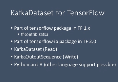
However, with the release of Tensorflow 2.0, the tables turned and the support for Apache Kafka data streaming module was issued along with support for a varied set of other data formats in the interest of the data science and statistics community (released in the IO package from Tensorflow: here).
Source: Kafka Summit NYC 2019, Yong Tang
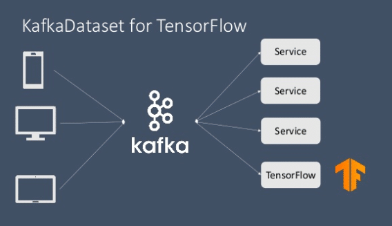
With this development, it is now possible to enable real time streaming with Kafka and Tensorflow with relative ease and minimized error. This process is implemented with the use of KafkaDataset module (written in C++) which is a part of the new release of the Tensorflow IO package. KafkaDataset module has been integrated as a subclass of tf.data.Dataset module. This module works just like any other data streaming module where users can simply read data from a kafka stream and use it in a Tensorflow graph or feed it to tf.keras and other Tensorflow specific modules for model training and evaluation purpose. The option of writing back through output stream is also possible of course.
Here is how to implement data streaming, processing, model training and inference gathering in just a few lines of code with Kafka support on Tensorflow:
Line 2 simply streams in data with the help of the KafkaDataset module and data processing and modeling are immediately commenced as can be seen in lines 3 and 4. Thereafter, we move on to the keras callback stage. Keras callbacks are very informative since they provide an overview of the internal stages and statistical details of the model during the training or prediction process. The callback function is written in the 7th line. The KafkaOutputSequence is responsible for writing the results to the output stream (with so much relative ease!). In line 13 the predict function is called to get the model details and inference on the test dataset.
Source: Kafka Summit NYC 2019, Yong Tang
Real time data streaming with Kafka and Tensorflow has not only helped in the elimination of the complicated infrastructure which previously bridged the wide gap between the two popular platforms, but has also made the process less error prone and more approachable for real time mission critical systems with respect to machine learning and data science. The above picture shows how easy it is now to implement Kafka along with Tensorflow with just one call for data streaming. Further development in this area looks highly promising and is sure to contribute manifold in the ease of scalability and smooth integration when it comes to Big Data, live or real time data streaming, machine learning and deep learning techniques to develop smart and autonomous systems across the globe!
Get a grip on the machine learning, data science, big data and several other intriguing topics by following our blogs or even our detailed courses provided in the links below:
Reports suggest that around 2.5 quintillion bytes of data are generated every single day. As the online usage growth increases at a tremendous rate, there is a need for immediate Data Science professionals who can clean the data, obtain insights from it, visualize it, train model and eventually come up with solutions using Big data for the betterment of the world.
By 2020, experts predict that there will be more than 2.7 million data science and analytics jobs openings. Having a glimpse of the entire Data Science pipeline, it is definitely tiresome for a single human to perform and at the same time excel at all the levels. Hence, Data Science has a plethora of career options that require a spectrum set of skill sets.
Let us explore the top 5 data science career options in 2019 (In no particular order).
1. Data Scientist
Data Scientist is one of the ‘high demand’ job roles. The day to day responsibilities involves the examination of big data. As a result of the analysis of the big data, they also actively perform data cleaning and organize the big data. They are well aware of the machine learning algorithms and understand when to use the appropriate algorithm. During the due course of data analysis and the outcome of machine learning models, patterns are identified in order to solve the business statement.
The reason why this role is so crucial in any organisation is that the company tends to take business decisions with the help of the insights discovered by the Data Scientist to have an edge over the company’s competitors. It is to be noted that the Data Scientist role is inclined more towards the technical domain. As the role demands a wide range of skill set, Data Scientists are one among the highest paid jobs.
Core Skills of a Data Scientist
Communication
Business Awareness
Database and querying
Data warehousing solutions
Data visualization
Machine learning algorithms
2. Business Intelligence Developer
BI Developer is a job role inclined more towards the Non-Technical domain but has a fair share of Technical responsibilities as well (if required) as a part of their day to day responsibilities. BI developers are responsible for creating and implementing business policies as a result of the insights obtained from the Technical team.
Apart from being a policymaker involving the usage of dedicated (or custom) Business Intelligence analytics tools, they will also have a fair share of coding in order to explore the dataset, present the insights of the dataset in a non-verbal manner. They help in bridging the gap between the technical team that works with the deepest technical understanding and the clients that want the results in the most non-technical manner. They are expected to generate reports from the insights and make it ‘less technical’ for others in the organisation. It is noted that the BI Developers have a deep understanding of Business when compared to Data Scientist.
Core Skills of a Business Analytics Developer
Business model analysis
Data warehousing
Design of business workflow
Business Intelligence software integration
3. Machine Learning Engineer
Once the data is clean and ready for analysis, the machine learning engineers work on these big data to train a predictive model that predicts the target variable. These models are used to analyze the trends of the data in the future so that the organisation can take the right business decisions. As the dataset involved in a real-life scenario would involve a lot of dimensions, it is difficult for a human eye to interpret insights from it. This is one of the reasons for training machine learning algorithms as it easily deals with such complex dataset. These engineers carry out a number of tests and analyze the outcomes of the model.
The reason for conducting constant tests on the model using various samples is to test the accuracy of the developed model. Apart from the training models, they also perform exploratory data analysis sometimes in order to understand the dataset completely which will, in turn, help them in training better predictive models.
Core Skills of Machine Learning Engineers
Machine Learning Algorithms
Data Modelling and Evaluation
Software Engineering
4. Data Engineer
The pipeline of any data-oriented company begins with the collection of big data from numerous sources. That’s where the data engineers operate in any given project. These engineers integrate data from various sources and optimize them according to the problem statement. The work usually involves writing queries on big data for easy and smooth accessibility. Their day to day responsibility is to provide a streamlined flow of big data from various distributed systems. Data engineering differs from the other data science careers as in, it is concentrated on the system and hardware that aids the company’s data analysis, rather than the analysis of data itself. They provide the organisation with efficient warehousing methods as well.
Core Skills of Data Engineer
Database Knowledge
Data Warehousing
Machine Learning algorithm
5. Business Analyst
Business Analyst is one of the most essential roles in the Data Science field. These analysts are responsible for understanding the data and it’s related trend post the decision making about a particular product. They store a good amount of data about various domains of the organisation. These data are really important because if any product of the organisation fails, these analysts work on these big data to understand the reason behind the failure of the project. This type of analysis is vital for all the organisations as it makes them understand the loopholes in the company. The analysts not only backtrack the loophole and in turn provide solutions for the same making sure the organisation takes the right decision in the future. At times, the business analyst act as a bridge between the technical team and the rest of the working community.
Core skills of Business Analyst
Business awareness
Communication
Process Modelling
Conclusion
The data science career options mentioned above are in no particular order. In my opinion, every career option in Data Science field works complimentary with one another. In any data-driven organization, regardless of the salary, every career role is important at the respective stages in a project.
Machine learning paradigm is ruled by a simple theorem known as “No Free Lunch” theorem. According to this, there is no algorithm in ML which will work best for all the problems. To state, one can not conclude that SVM is a better algorithm than decision trees or linear regression. Selection of an algorithm is dependent on the problem at hand and other factors like the size and structure of the dataset. Hence, one should try different algorithms to find a better fit for their use case
In this blog, we are going to look into the top machine learning algorithms. You should know and implement the following algorithms to find out the best one for your use case
Top 10 Best Machine Learning Algorithms
1. Linear Regression
Regression is a method used to predict numerical numbers. Regression is a statistical measure which tries to determine the power of the relation between the label-related characteristics of a single variable and other factors called autonomous (periodic attributes) variable. Regression is a statistical measure. Just as the classification is used for categorical label prediction, regression is used for ongoing value prediction. For example, we might like to anticipate the salary or potential sales of a new product based on the prices of graduates with 5-year work experience. Regression is often used to determine how the cost of an item is affected by specific variables such as product cost, interest rates, specific industries or sectors.
The linear regression tries by a linear equation to model the connection between a scalar variable and one or more explaining factors. For instance, using a linear regression model, one might want to connect the weights of people to their heights
The driver calculates a linear pattern of regression. It utilizes the model selection criterion Akaike. A test of the comparative value of fitness to statistics is the Akaike information criterion. It is based on the notion of entropy, which actually provides a comparative metric of data wasted when a specified template is used to portray the truth. The compromise between bias and variance in model building or between the precision and complexity of the model can be described.
2. Logistic Regression
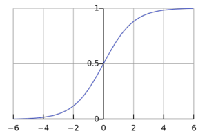
Logistic regression is a classification system that predicts the categorical results variable that may take one of the restricted sets of category scores using entry factors. A binomial logistical regression is restricted to 2 binary outputs and more than 2 classes can be achieved through a multinomial logistic regression. For example, classifying binary conditions as’ safe’/’don’t-healthy’ or’ bike’ /’ vehicle’ /’ truck’ is logistic regression. Logistic regression is used to create an information category forecast for weighted entry scores by the logistic sigmoid function.
The probability of a dependent variable based on separate factors is estimated by a logistic regression model. The variable depends on the yield that we want to forecast, whereas the indigenous variables or explaining variables may affect the performance. Multiple regression means an assessment of regression with two or more independent variables. On the other side, multivariable regression relates to an assessment of regression with two or more dependent factors.
3. Linear Discriminant Analysis
Logistic regression is traditionally a two-class classification problem algorithm. If you have more than two classes, the Linear Discriminant Analysis algorithm is the favorite technique of linear classification. It contains statistical information characteristics, which are calculated for each category.
For a single input variable this includes:
The mean value for each class.
The variance calculated across all classes.
The predictions are calculated by determining a discriminating value for each class and by predicting the highest value for each class. The method implies that the information is distributed Gaussian (bell curve) so that outliers are removed from your information in advance. It is an easy and strong way to classify predictive problem modeling.
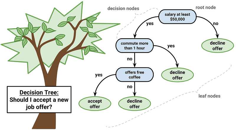
4. Classification and Regression Trees
Prediction Trees are used to forecast answer or YY class of X1, X2,…, XnX1,X2,… ,Xn entry. If the constant reaction is called a regression tree, it is called a ranking tree, if it is categorical. We inspect the significance of one entry XiXi at any point of the tree and proceed to the left or to the correct subbranch, based on the (binary) response. If we hit a tree, we will discover the forecast (generally the leaves as the most popular value of the accessible courses is a straightforward statistical figure of the dataset). In contrast to global model linear or polynomial regression (a predictive formula should be contained in the whole data space), trees attempt to split the data space in a sufficiently small part, where a simply different model can be applied on each side. For each xx information, the non-leaf portion of the tree is simply the process to determine what model we use for the classification of each information (i.e. which leaf).
5. Naive Bayes
A Naive Bayes classification is a supervised algorithm for machinery-learning which utilizes the theorem of Bayes, which implies statistical independence of its characteristics. The theorem depends on the naive premise that input factors are autonomous from each other, that is, that when an extra variable is provided there is no way to understand anything about other factors. It has demonstrated to be a classifier with excellent outcomes regardless of this hypothesis. The Bavarian Theorem, relying on a conditional probability, or in easy words, is used for the Naive Bayes classifications as a probability of a case (A) occurring considering that another incident (B) has already occurred. In essence, the theorem enables an update of the hypothesis every moment fresh proof is presented.
The equation below expresses Bayes’ Theorem in the language of probability:
Let’s explain what each of these terms means.
“P” is the symbol to denote probability.
P(A | B) = The probability of event A (hypothesis) occurring given that B (evidence) has occurred.
P(B | A) = The probability of the event B (evidence) occurring given that A (hypothesis) has occurred.
P(A) = The probability of event B (hypothesis) occurring.
P(B) = The probability of event A (evidence) occurring.
6. K-Nearest Neighbors
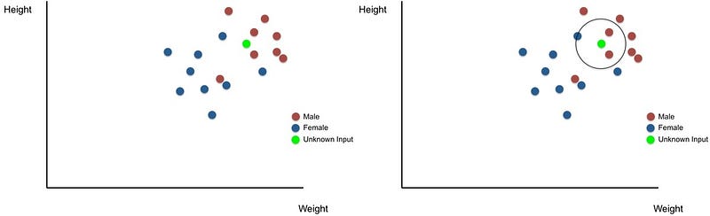
The KNN is a simple machine study algorithm which classifies an entry using its closest neighbours. The input of information points of particular males and women’s height and weight as shown below should be provided, for instance, by a k-NN algorithm. K-NN can peer into the closest k neighbour (personal) and determine if the entry gender is masculine in order to determine the gender of an unidentified object (green point). This technique is extremely easy and logical, with a strong achievement level for labelling unidentified input.
k-NN is used in a range of machine learning tasks; k-NN, for example, can help in computer vision in hand-written letters and the algorithm is used to identify genes that are contributing to a specific characteristic of the gene expression analysis. Overall, neighbours close to each other offer a mixture of ease and efficiency that makes it an appealing algorithm for many teaching machines.7. Learning Vector Quantization
8. Bagging and Random Forest
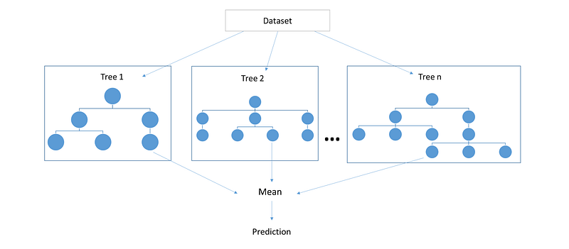
A Random Forest is a group of easy tree predictors, each of which is capable of generating an answer when it has a number of predictor values. This reaction requires the form of a class affiliation for classification issues, which combines or classifies a number of indigenous predictor scores with one of the classifications in the dependent variable. Otherwise, the tree reaction is an assessment of the dependent variable considering the predictors for regression difficulties. Breiman has created the Random Forest algorithm.
An arbitrary amount of plain trees are a random forest used to determine the ultimate result. The ensemble of easy trees votes for the most common category for classification issues. Their answers are averaged to get an assessment of the dependent variable for regression problems. With tree assemblies, the forecast precision (i.e. greater capacity to detect fresh information instances) can improve considerably.
9. SVM
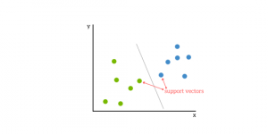
The support vector machine(SVM) is a supervised, classifying, and regressing machine learning algorithm. In classification issues, SVMs are more common, and as such, we shall be focusing on that article.SVMs are based on the idea of finding a hyperplane that best divides a dataset into two classes, as shown in the image below.
You can think of a hyperplane as a line that linearly separates and classifies a set of data.
The more our information points are intuitively located from the hyperplane, the more assured that they have been categorized properly. We would, therefore, like to see as far as feasible from our information spots on the right hand of the hyperplane.
So when new test data are added, the class we assign to it will be determined on any side of the hyperplane.
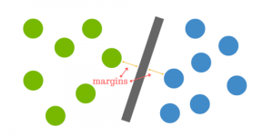
The distance from the hyperplane to the nearest point is called the margin. The aim is to select a hyperplane with as much margin as feasible between the hyperplane and any point in the practice set to give fresh information a higher opportunity to be properly categorized.
But the data is rarely ever as clean as our simple example above. A dataset will often look more like the jumbled balls below which represent a linearly non-separable dataset.
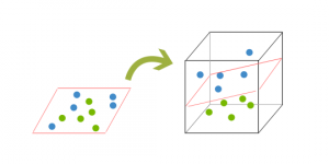
It is essential to switch from a 2D perspective to a 3D perspective to classify a dataset like the one above. Another streamlined instance makes it easier to explain this. Imagine our two balls stood on a board and this booklet is raised abruptly, throwing the balls into the air. You use the cover to distinguish them when the buttons are up in the air. This “raising” of the balls reflects a greater identification of the information. This is known as kernelling.
Our hyperplanes can be no longer a row because we are in three dimensions. It should be a flight now, as shown in the above instance. The concept is to map the information into greater and lower sizes until a hyperplane can be created to separate the information.
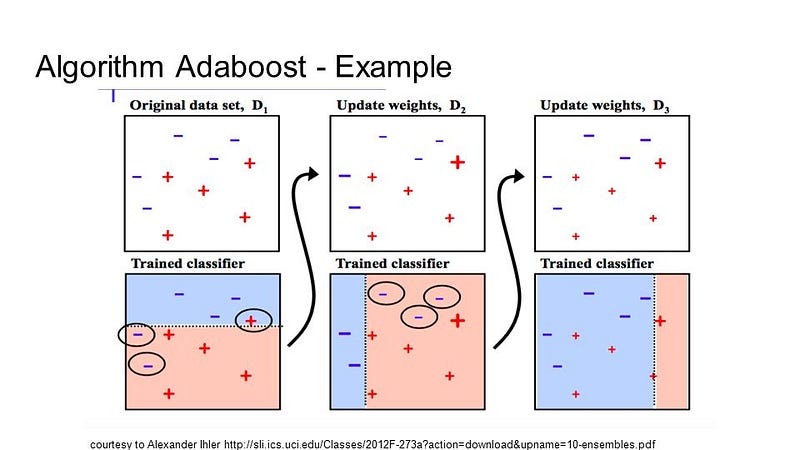
10. Boosting and AdaBoost
Boosting is an ensemble technology which tries to build a powerful classification of a set of weak classifiers. This is done using a training data model and then a second model has created that attempts the errors of the first model to be corrected. Until the training set is perfectly predicted or a maximum number of models are added, models are added.
AdaBoost was the first truly effective binary classification boosting algorithm. It is the best point of start for improvement. Most of them are stochastic gradient boosters, based on AdaBoost modern boosting techniques.
With brief choice trees, AdaBoost is used. After the creation of the first tree, each exercise instance uses the performance of the tree to weigh how much attention should be given to the next tree to be built. Data that are difficult to forecast will be provided more weight, while cases that are easily predictable will be less important. Sequentially, models are produced one by one to update each of the weights on the teaching sessions which impact on the study of the next tree. After all, trees have been produced, fresh information are predicted and how precise it was on the training data weighs the efficiency of each tree.
Since the algorithm is so careful about correcting errors, it is essential that smooth information is deleted with outliers.
Summary
In the end, every beginner in data science has one basic starting questions that which algorithm is best for all the cases. The response to the issue is not straightforward and depends on many factors like information magnitude, quality and type of information; time required for computation; the importance of the assignment; and purpose of information
Even an experienced data scientist cannot say which algorithm works best before distinct algorithms are tested. While many other machine learning algorithms exist, they are the most common. This is a nice starting point to understand if you are a beginner for machine learning.
Data science is one of the hottest topics in the 21st century because we are generating data at a rate which is much higher than what we can actually process. A lot of business and tech firms are now leveraging key benefits by harnessing the benefits of data science. Due to this, data science right now is really booming.
In this blog, we will deep dive into the world of machine learning. We will walk you through machine learning basics and have a look at the process of building an ML model. We will also build a random forest model in python to ease out the understanding process.
What is Machine Learning?
Machine Learning is the science of getting computers to learn and act like humans do, and improve their learning over time in an autonomous fashion, by feeding them data and information in the form of observations and real-world interactions.
There are many different types of machine learning algorithms, with hundreds published each day, and they’re typically grouped by either learning style (i.e. supervised learning, unsupervised learning, semi-supervised learning) or by similarity in form or function (i.e. classification, regression, decision tree, clustering, deep learning, etc.). Regardless of learning style or function, all combinations of machine learning algorithms consist of the following:
Representation (a set of classifiers or the language that a computer understands)
Evaluation (aka objective/scoring function)
Optimization (search method; often the highest-scoring classifier, for example; there are both off-the-shelf and custom optimization methods used)
Steps for Building ML Model
Here is a step-by-step example of how a hospital might use machine learning to improve both patient outcomes and ROI:
1. Define Project Objectives
The first step of the life cycle is to identify an opportunity to tangibly improve operations, increase customer satisfaction, or otherwise create value. In the medical industry, discharged patients sometimes develop conditions that necessitate their return to the hospital. In addition to being dangerous and troublesome for the patient, these readmissions mean the hospital will spend additional time and resources on treating patients for the second time.
2. Acquire and Explore Data
The next step is to collect and prepare all of the relevant data for use in machine learning. This means consulting medical domain experts to determine what data might be relevant in predicting readmission rates, gathering that data from historical patient records, and getting it into a format suitable for analysis, most likely into a flat file format such as a .csv.
3. Model Data
In order to gain insights from your data with machine learning, you have to determine your target variable, the factor of which you are trying to gain a deeper understanding. In this case, the hospital will choose “readmitted,” which is included as a feature in its historical dataset during data collection. Then, they will run machine learning algorithms on the dataset that build models that learn by example from the historical data. Finally, the hospital runs the trained models on data the model hasn’t been trained on to forecast whether new patients are likely to be readmitted, allowing it to make better patient care decisions.
4. Interpret and Communicate
One of the most difficult tasks of machine learning projects is explaining a model’s outcomes to those without any data science background, particularly in highly regulated industries such as healthcare. Traditionally, machine learning has been thought of as a “black box” because of how difficult it is to interpret insights and communicate their value to stakeholders and regulatory bodies alike. The more interpretable your model, the easier it will be to meet regulatory requirements and communicate its value to management and other key stakeholders.
5. Implement, Document, and Maintain
The final step is to implement, document, and maintain the data science project so the hospital can continue to leverage and improve upon its models. Model deployment often poses a problem because of the coding and data science experience it requires, and the time-to-implementation from the beginning of the cycle using traditional data science methods is prohibitively long.
Problem Statement
A certain car manufacturing company X is looking to target its customers for their particular car model. Customers are identified by their age, salary, and Gender. The organisation wants to identify or predict which customers will affect the sales of their new car and actually purchase it.
We have a purchased column here which holds two values i.e 0 and 1. 0 indicates that the car has not been purchased by a certain individual. 1 indicates the sale of the car.
Code Implementation
Importing the Required Libraries
You need to import all the required libraries first which will ease the model building parts for us. We are using keras to build our random forest model. We are using the matplotlib library to plot the charts and graphs and visualise results. In the end, we are also importing functions from the sklearn module which can help us in splitting our data into training and testing parts
# Importing the libraries
import numpy as np
import matplotlib.pyplot as plt
import pandas as pd
from sklearn.model_selection import train_test_split
from sklearn.ensemble import RandomForestClassifier
Loading the Dataset
In this step, you need to load your dataset in the memory. After that, we separate out the dependent and the independent variables for the training of our classifier. In most of the cases, you need to separate the dependent and he the independent variables
# Importing the dataset
dataset = pd.read_csv('Social_Network_Ads.csv')
X = dataset.iloc[:, [2, 3]].values
y = dataset.iloc[:, 4].values
Splitting the Dataset to Form Training and Test Data
In all the cases, you need to make some partitions in your data. A major chunk of your data acts as a training set and a smaller chunk acts as a test set. There are no clearly defined criteria on the proportion of the training and the test set. But most people follow 70–30 or 75–25 rule where a larger chunk is your training set. We train the data on the training set and test it on the test set. This process is known as validation. The prime idea behind this purpose is that one needs to gauge the performance of the model on the data which model has never seen before. In the real-world scenarios, the model will be predicting values on the unseen data. Furthermore, techniques like validation help us in avoiding overfitting or underfitting the model.
Overfitting refers to the case when our model has learnt all about the specific data on which it trained. It will work well on the training data but will have poor accuracy for any unseen data point. Overfitting is like your model is very specific to the data it has and has no generality. Similarly, underfitting is the case where your model is very general and is not able to predict well for your specific use-case. To achieve the best model accuracy, you need to strike a perfect balance between overfitting and under-fitting.
# Splitting the dataset into the Training set and Test set
from sklearn.model_selection import train_test_split
X_train, X_test, y_train, y_test = train_test_split(X, y, test_size = 0.25, random_state = 0)
In this case, we are fitting our model with the training data. We are using the random forest model exposed by the sklearn package in python. Ultimately, we pass the dependent and independent features separately through which our model makes an internal mapping between them using mathematical coefficients.
# Fitting Random Forest Classification to the Training set
from sklearn.ensemble import RandomForestClassifier
classifier = RandomForestClassifier(n_estimators = 10, criterion = 'entropy', random_state = 0)
classifier.fit(X_train, y_train)
Predicting Results from the Classifier
In this part, we are passing unseen values to our model on which it is making predictions. We use a confusion matrix to derive metrics like accuracy, precision, and recall for our model. These metrics help us to understand the performance of the model.
# Predicting the Test set results
y_pred = classifier.predict(X_test)

# Making the Confusion Matrix
from sklearn.metrics import confusion_matrix
cm = confusion_matrix(y_test, y_pred)
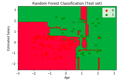
Visualising the Predictions
Additionally, we have made an attempt to visualise the predictions of our model using the below code.
# Visualising the Test set results
# Visualising the Test set results
from matplotlib.colors import ListedColormap
X_set, y_set = X_test, y_test
X1, X2 = np.meshgrid(np.arange(start = X_set[:, 0].min() - 1, stop = X_set[:, 0].max() + 1, step = 0.01),
                     np.arange(start = X_set[:, 1].min() - 1, stop = X_set[:, 1].max() + 1, step = 0.01))
plt.contourf(X1, X2, classifier.predict(np.array([X1.ravel(), X2.ravel()]).T).reshape(X1.shape),
             alpha = 0.75, cmap = ListedColormap(('red', 'green')))
plt.xlim(X1.min(), X1.max())
plt.ylim(X2.min(), X2.max())
for i, j in enumerate(np.unique(y_set)):
    plt.scatter(X_set[y_set == j, 0], X_set[y_set == j, 1],
                c = ListedColormap(('red', 'green'))(i), label = j)
plt.title('Random Forest Classification (Test set)')
plt.xlabel('Age')
plt.ylabel('Estimated Salary')
plt.legend()
plt.show()
Summary
Hence, in this Machine Learning Tutorial, we studied the basics of ML. Earlier machine learning was the theory that computers can learn without being programmed to perform specific tasks. But now, the researchers interested in artificial intelligence wanted to see if computers could learn from data. They learn from previous computations to produce reliable decisions and results. It’s a science that’s not new — but one that’s gaining fresh momentum.
Follow this link, if you are looking to learn more about data science online!