Building data pipelines is a core component of data science at a startup. In order to build data products, you need to be able to collect data points from millions of users and process the results in near real-time. Today, many organizations nowadays are struggling with the quality of their data. Data quality (DQ) problems can arise in various ways. Here are common causes of bad data quality:
Multiple data sources: Multiple sources with the same data may produce duplicates; a problem of consistency.
Limited computing resources: Lack of sufficient computing resources and/or digitalization may limit the accessibility of relevant data; a problem of accessibility.
Changing data needs: Data requirements change on an ongoing basis due to new company strategies or the introduction of new technologies; a problem of relevance.
Different processes using and updating the same data; a problem of consistency.
In this blog, we are going to look into the world of data lakes and their significance. Furthermore, we will peep into some of the inherent issues in data lakes like quality management. In the end, we will discuss some of the quality measures to control the quality of data in data lakes.
What is Data Lake?
A data lake is a centralized place, like a lake, that allows you to hold a lot of raw data in its native format, structured and unstructured, at any scale. Furthermore, you can store your data as- it is, without having to first structure the data or define it until its needed. Its purpose is for creating reporting dashboards and visualizations, real-time analytics, and machine learning. Also, this can guide better programmatic advertising decisions.
In its extreme form, a data lake ingests data in its raw, original state, straight from data sources. This happens without any cleansing, standardization, remodelling, or transformation. These and other sacrosanct data management disciplines are applicable on the fly. Moreover, it helps in enabling ad hoc queries, data exploration, and discovery-oriented analytics. The early ingestion of data means that operational data is present and made available to analytics as soon as possible. Additionally, the raw state of the data ensures that data analysts, data scientists, and similar users have ample raw material. They can repurpose into many diverse data sets, as needed by unanticipated analytics questions.
Components of Data Lake
A Data Lake is a platform combining a number of advanced, complex data storage and data analysis technologies.
To simplify, we might group the components of a Data Lake into four categories, representing the four stages of data management:
Data Ingestion and Storage, that is the capability of acquiring data in real time or in batch, and also the capacity to store data and make it accessible.
Data Processing, that is the ability to work with raw data so that they’re ready to be analysed through standard processes. It also includes the capability of engineering solutions that extract value from the data, leveraging automated, periodical processes resulting from the analysis operations.
Data Analysis, that is the creation of modules that extract insights from data in a systematic manner; this can happen in real time or by means of processes that are running periodically.
Data Integration, that is the ability to connect applications to the platform; in the first place, applications must allow querying the Data Lake to extract the data in the right format, based on the usage you want to make of it
Why use Data Lakes
1. Data Indexing
Data Lakes allow you to store relational data (a collection of data items organized as a set of formally-described tables from which data can be accessed or reassembled in many different ways without having to reorganize the database tables.) — operational databases (data collected in real-time), and data from line of business applications, and non-relational data like mobile apps, connected devices, and social media. They also give you the ability to understand what data is in the lake through crawling, cataloguing, and indexing of data.
2. Analytics
Data Lakes allow data scientists, data developers, and operations analysts to access data with their choice of analytic tools and frameworks. This also includes open source data frameworks such as Apache Hadoop, Presto, and Apache Spark, and commercial offerings from data warehouse and business intelligence vendors. Data Lakes allow you to run Analytics without the need to move your data from one system to another.
3. Machine Learning
Data Lakes will allow organizations to generate different types of marketing and operational insights. It includes reporting on historical data and doing machine learning where models produce forecasts and predictions.
4. Improved Customer Interaction
A Data Lake can combine customer data from a CRM platform with social media data analytics, as well as a marketing platform that includes buying history to empower the business to understand the most profitable audiences, the root of customer churn, and what promotions or rewards could increase loyalty.
The Challenge with Data Lakes
A challenge in data lakes is the inability for analysts to determine data quality because a thorough check-up has not taken place. Also, there is no way to use insights from others who have worked with the data, as there is no account of the lineage of findings by previous analysts. Finally, one of the biggest risks of data lakes is security and access control. Data can be placed into a lake without any oversight, and some of the data may contain privacy and regulatory requirements that other data doesn’t.
Ways to Improve Quality in Data Lakes
1. Use of Machine Learning and NLP
Machine learning can be a game changer because it can capture tacit knowledge from the people that know the data best, then turn this knowledge into algorithms, which can be used to automate data processing at scale. This is exactly how Talend is leveraging Spark machine learning to learn from data stewards during data matching and deduplication of data samples, and then apply it at big data scale for billions of records.
2. Setting the standards for agile data quality
for companies to get the most out of their digital transformation projects and build an agile data lake, they need to design data quality processes from the start. Organisations should focus on standardising the following for maintaining the quality of big data
Roles — Identify roles including data stewards and users of data
Discovery — Understand where data is coming from, where it is going and what shape it is in. Focus on cleaning your most valuable and most used data first
Standardization — Validate, cleanse, and transform data. Add metadata early so data can be found by humans and machines. Identify and protect personal and private organizational data with data masking.
Reconciliation — Verify that data was migrated correctly
Self-service — Make data quality agile, by letting people who know the data best, clean their data
Automate — Identify where machine learning in the data quality process can help, such as data deduplication
Monitor and Manage — Get continuous feedback from users, come up with data quality measurement metrics to improve
3. Employing data quality management frameworks
Another category of frameworks focuses on the maturity of data quality management processes. They aim at assessing the maturity level of DQ management to understand best practices in mature organizations and identify areas for improvement. Popular examples of such frameworks include Total Data Quality Management (TDQM), Capability Maturity Model Integration (CMMI), Control Objectives for Information and Related Technology (CobiT), Information Technology Infrastructure Library (ITIL), and Six Sigma.
As an example, we can take the TDQM framework. A TDQM cycle consists of four steps, Define, Measure, Analyze, and Improve. The define step identifies the pertinent data quality dimensions. One can quantify them using metrics in the Measure step. Some example metrics are the percentage of customer records with the incorrect address (accuracy), the percentage of customer records with missing birth date (completeness), or an indicator specifying the last update of the customer. The Analyze step tries to identify the root cause of data quality problems. We remedy the previous issues in the improve step. Example actions could be automatic and periodic verification of customer addresses, the addition of a constraint that makes the birth date a mandatory data field, and the generation of alerts when there is no update to customer data in 6 months.
Summary
More and more companies are experimenting with data lakes, hoping to capture inherent advantages in information streams that are readily accessible regardless of platform and business case and that cost less to store than do data in traditional warehouses. As with any deployment of new technology, however, companies will need to reimagine systems, processes, and governance models. Furthermore, if actual data quality improvement is not an option in the short term for reasons of technical constraints or strategic priorities, it is sometimes a partial solution to annotate the data with explicit information about its quality. Such data quality metadata can be stored in the catalogue, possibly with other metadata.
Follow this link, if you are looking to learn more about data science online!
Machine Learning is the word of the mouth for everyone involved in the analytics world. Gone are those days of the traditional manual approach of taking key business decisions. Machine Learning is the future and is here to stay.
However, the term Machine Learning is not a new one. It was there since the advent of computers but has grown tremendously in the last decade due to the massive amounts of data that’s getting generated, and the enormous computational power that modern-day system possesses.
Machine Learning is the art of Predictive Analytics where a system is trained on a set of data to learn patterns from it and then tested to make predictions on a new set of data. The more accurate the predictions are, the better the model performs. However, the metric for the accuracy of the model varies based on the domain one is working in.
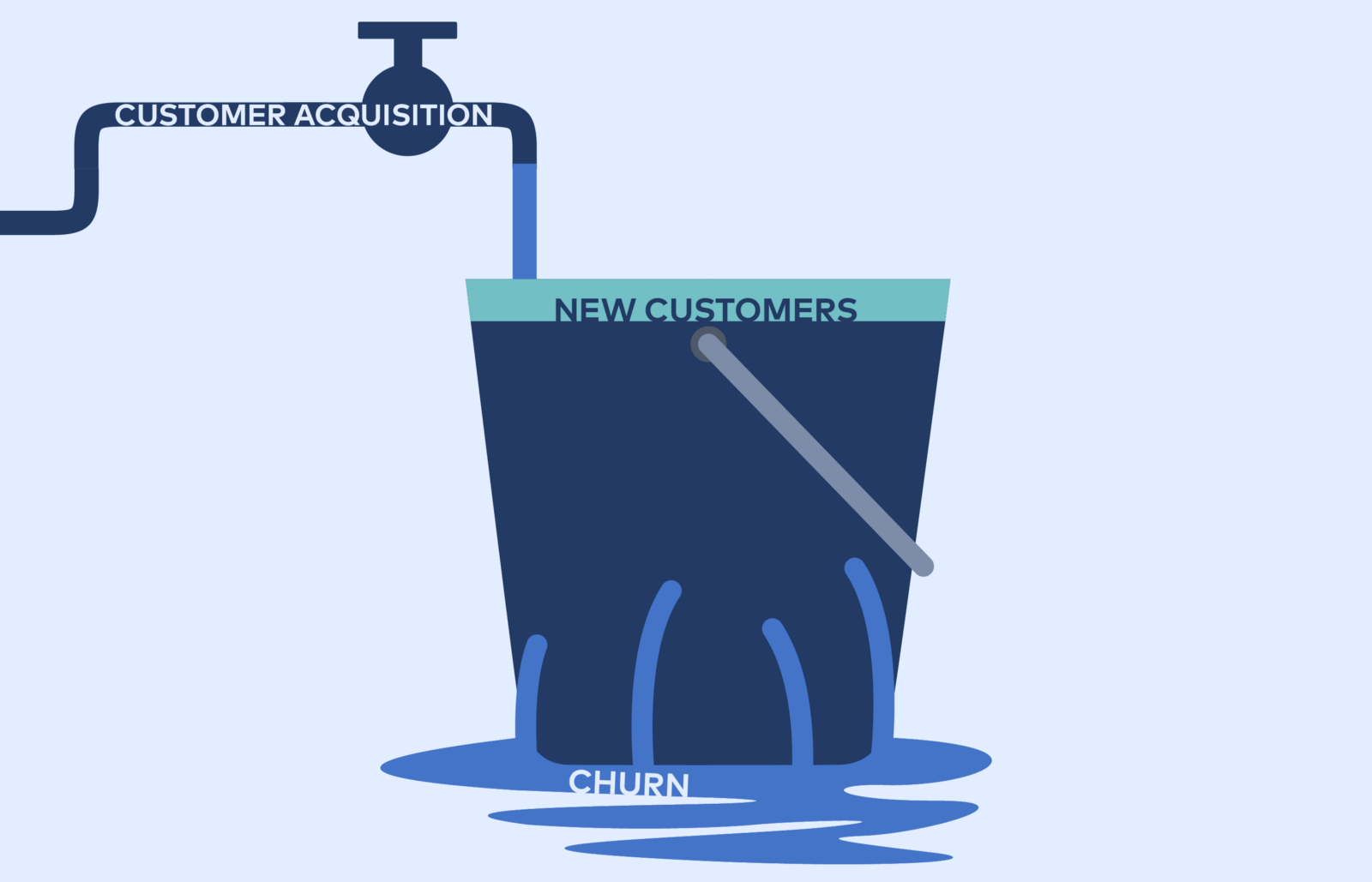
Predictive Analytics has several usages in the modern world. It has been implemented in almost all sectors to make better business decisions and to stay ahead in the market. In this blog post, we would look into one of the key areas where Machine Learning has made its mark is the Customer Churn Prediction.
What is Customer Churn?
For any e-commerce business or businesses in which everything depends on the behavior of customers, retaining them is the number one priority for the organization. Customer churn is the process in which the customers stop using the products or services of a business.
Customer Churn or Customer Attrition is a better business strategy than acquiring the services of a new customer. Retaining the present customers is cost-effective, and a bit of effort could regain the trust that the customers might have lost on the services.
On the other hand, to get the service of the new customer, a business needs to spend a lot of time, and money on to the sales, and marketing department, more lucrative offers, and most importantly earning their trust. It would take more recourses to earn the trust of a new customer than to retain the existing one.
What are the Causes of Customer Churn?
There is a multitude of reasons why a customer could decide to stop using the services of a company. However, a couple of such reasons overwhelms others in the market.
Customer Service – This is one of the most important aspects on which business the growth of a business depends. Any customer could leave the services of a company if it’s poor or doesn’t live up to the expectations. A study showed that nearly ninety percent of the customer leave due to poor experience as modern era deems exceptional services, and experiences.
When a customer doesn’t receive such eye-catching experience from a business, it tends to lean towards its competitors leaving behind negative reviews in various social media from their past experiences which also stops potential new customers from using the service. Another study showed that almost fifty-nine percent of the people aged between twenty-five, and thirty share negative client experiences online.
Thus, poor customer experience not only results in the loss of a single customer but multiple customers as well which hinders the growth of the business in the process.
Onboarding Process – Whenever the business is looking to attract a new customer to use their service, it is necessary that the on-boarding process which includes timely follow-ups, regular communications, updates about new products, and so on are being followed, and maintained consistently over a period of time.
What are some of the Disadvantages of Customer Churn?
A customer’s lifetime value and the growth of the business maintains a direct relationship between each other i.e., more chances that the customer would churn, the less is the potential for the business to grow. Even a good marketing strategy would not save a business if it continues to lose customers at regular intervals due to other reasons and spend more money on acquiring new customers who are not guaranteed to be loyal.
There is a lot of debate surrounding customer churn and acquiring new customers because the former is much more cost-effective and ensures business growth. Thus companies spend almost seven times more effort, and time to retain old customers than acquire a new one. The global value of a customer lost is nearly two hundred, and forty-three dollars which makes churning a costly affair for any business.
What Strategies could a Business Undertake to prevent Customer Churn?
Customer Churn hinders or prevents the growth of an organization. Thus it is necessary that any business or organization has a flexible system in place to prevent the churn of customers and ensure its growth in the process. The companies need to find the metrics to identify the probability of a customer leaving, and chalk out strategies for improvement of its services, and products.
The calculation of the possibility of the customer churning varies from one business to another. There is no one fixed methodology that every organization uses to prevent churn. A churn rate could represent a variety of things such as – the total number of customers lost, the cost of the business loss, what percentage of the customers left in comparison to the total customer count of the organization, and so on.
Improving the customer experience should be the first strategy on the agenda of any business to prevent churn. Apart from that, marinating customer loyalty by providing better, personalized services is another important step one could undertake. Additionally, many organizations sent out customer survey time, and again to keep track of their customer experiences, and also seek reasons from them who have already churned.
A company should understand and learn about its customers beforehand. The amount of data that’s available all over the internet is sufficient to analyze a customer’s behavior, his likes, and dislikes, and improve the services based on their needs. All these measures, if taken with utmost care could help a business prevent its customers from churning.
Telecom Customer Churn Prediction
Previously, we learned how Predictive Analytics is being employed by various businesses to prevent any event from occurring and reduce the chances of losing by putting the right system in place. As customer churn is a global issue, we would now see how Machine Learning could be used to predict the customer churn of a telecom company.
Gender – Determines whether the customer is a male or a female.
Senior Citizen – A binary variable with values as 1 for senior citizen and 0 for not a senior citizen.
Partner – Values as ‘yes’ or ‘no based on whether the customer has a partner.
Dependents – Values as ‘yes’ or ‘no’ based on whether the customer has dependents.
Tenure – A numerical feature which gives the total number of months the customer stayed with the company.
Phone Service – Values as ‘yes’ or ‘no’ based on whether the customer has phone service.
Multiple Lines – Values as ‘yes’ or ‘no’ based on whether the customer has multiple lines.
Internet Service – The internet service providers the customer has. The value is ‘No’ if the customer doesn’t have internet service.
Online Security – Values as ‘yes’ or ‘no’ based on whether the customer has online security.
Online Backup – Values as ‘yes’ or ‘no’ based on whether the customer has online backup.
Device Protection – Values as ‘yes’ or ‘no’ based on whether the customer has device protection.
Tech Support – Values as ‘yes’ or ‘no’ based on whether the customer has tech support.
Streaming TV – Values as ‘yes’ or ‘no’ based on whether the customer has a streaming TV.
Streaming Movies – Values as ‘yes’ or ‘no’ based on whether the customer has streaming movies.
Contract – This column gives the term of the contract for the customer which could be a year, two years or month-to-month.
Paperless Billing – Values as ‘yes’ or ‘no’ based on whether the customer has a paperless billing.
Payment Method – It gives the payment method used by the customer which could be a credit card, Bank Transfer, Mailed Check, or Electronic Check.
Monthly Charges – This is the total charge incurred by the customer monthly.
Total Charges – The value of the total amount charged.
Churn – This is our target variable which needs to be predicted. Its values are either Yes (if the customer has churned), or No (if the customer is still with the company)
The following steps are the walkthrough of the code which we have written to predict the customer churn.
First, we have imported all the necessary libraries we would need to proceed further in our code
Just to get an idea of how our data looks likes, we have read the CSV file and printed out the first five rows of our data in the form of a data frame
Once, the data is read, some pre-processing needed to be done to check for null, outliers, and so on
Once the pre-processing is done, the next step is to get the relevant features to use in our model for the prediction. For that, we have done some data visualization to find out the relevancy of each predictor variables
After the data has been plotted, it is observed that Gender doesn’t have much influence on churn, whereas senior citizens are more likely to leave the company. Also, Phone Service has more influence on Churn than Multiple Lines
A model cannot take categorical data as input, hence those features are encoded into numbers to be used in our prediction
Based on our observation, we have taken the features which have more influence on churn prediction
The data is scaled, and split it into train and test set
We have fitted the Random Forest classifier to our new scaled data
Predicted the result and using the confusion matrix as the metric for our model
The model gives us (1155 + 190 = 1345) correct predictions and (273 + 143 = 416) incorrect predictions
The entire code could be found in this GitHub link
Conclusion
We have built a basic Random Forest Classifier model to predict the Customer Churn for a telecom company. The model could be improved with further manipulation of the parameters of the classifier and also by applying different algorithms.
Dimensionless has several resources to get started with.
The advancement in the analytical eco-space has reached new heights in the recent past. The emergence of new tools and techniques has certainly made life easier for an analytics professional to play around with the data. Moreover, the massive amounts of data that’s getting generated from diverse sources need huge computational power and storage system for analysis.
Three of the most commonly used terms in analytics are Data mining, Machine Learning, and Data Science which is a combination of both. In this blog post, we would look into each of these three buzzwords along with examples.
Data Mining:
By term ‘mining’ we refer to extracting some object by digging. Similarly, that analogy could be applied to data where information could be extracted by digging into it. Data mining is one of the most used terms these days. Unlike previously, our life is circulated entirely by big data and we have the tools and techniques to handle such voluminous diverse meaningful data.
In the data, there are a lot of patterns which people could discover once the data has been gathered from relevant sources. The hidden patterns could be extracted to provide valuable insights by combining multiple sources of data even if it is junk. This entire process is known as Data mining.
Now the data used for mining could be enterprise data which are restricted and secured and has privacy issues. It could also be an integration of multiple sources which includes financial data, third-party data, etc. The more the data available to us, the better it is as we need to find patterns and insights in sequential and non-sequential data.
The steps involved in data mining are –
Data Collection – This is one of the most important steps in Data mining as getting the correct data is always a challenge in any organization. To find patterns in the data, we need to ensure that the source of the data is accurate and as much as possible data is gathered.
Data Cleaning – A lot of the times the data we get is not clean enough to draw insights from it. There could be missing values, outliers, NULL in the data which needs to be handled either by deletion or by imputation based on its significance to the business.
Data Analysis – Once the data is gathered, and cleaned the next step is to analyze the data which in short known as Exploratory Data Analysis. Several techniques and methodologies are applied in this step to derive relevant insights from the data.
Data Interpretation – Only analyzing the data is worthless unless it is interpreted through the form of graphs or charts to the stakeholders or the business who would make conclusions based on the analysis.
Data mining has several usages in the real world. For example, if we take the logs data for login in a web application, we would see that the data is messy containing information like timestamp, activities of the user, time spent on the website, etc. However, if we clean the data, and then analyze it, we would find some relevant information from it such as the user’s regular habit, the peak time for most of the activities, and so on. All this information could help to increase the efficiency of the system.
Another example of data mining is in crime prevention. Though data mining has most usage in education and healthcare, it is also used by agencies in the crime department to spot patterns in the data. This data would consist of information about some of the criminal activities that have taken place. Hence, mining, and gathering information from the data would help the agencies to predict future crime events and prevent it from occurring. The agencies could mine the data and find out the place where the next crime could take place. They could also prevent cross-border calamity by understanding which vehicle to check, the age of the occupants, etc.
However, a few of the important points one should remember about Data Mining –
Data mining should not be considered as the first solution to any analysis task if other accurate solutions are applicable. It should be used when such solutions fail to provide value.
Sufficient amount of data should be present to draw insights from it.
The problem should be understood to be a Regression or a Classification one.
Machine Learning:
Previously, we learned about Data mining which is about gathering, cleaning, analyzing, and interpreting relevant insights from the data for the business to draw conclusions from it.
If Data mining is about describing a set of events, Machine Learning is about predicting the future events. It is the term coined to define a system which learns from past data to generalize and predict the future events from the unknown set of data.
Machine Learning could be divided into three categories –
Supervised Learning – In supervised learning, the target is labeled i.e., for every corresponding row there is an output value.
Unsupervised Learning – The data set is unlabelled in unsupervised learning i.e., one has to cluster the data into various groups based on the similarities in the pattern of the data points.
Reinforcement Learning – It is a special category of Machine Learning which is mostly used in self-driving cars. In reinforcement learning, the learner is rewarded for every correct move, and penalized for any incorrect move.
The field of Machine Learning is vast, and it requires a blend of statistics, programming, and most importantly data intuition to master it. Supervised and unsupervised learning are used to solve regression, classification, and clustering problems.
In regression problems, the target is numeric i.e., continuous or discrete in nature. A continuous value could be an integer, float, or a decimal, whereas a discrete value is a number or an integer.
In classification problems, the target is categorical i.e., binary, multinomial, or ordinal in nature.
In clustering problems, the dataset is grouped into different clusters based on the similar properties among the data in a particular group.
Machine Learning has a vast usage in various fields such as Banking, Insurance, Healthcare, Manufacturing, Oil and Gas, and so on. Professionals from various disciplines feel the need to predict future outcomes in order to work efficiently and prepare for the best by taking appropriate actions. Some of the real-life examples where Machine Learning has found its usage is –
Email Spam filtering – This is the first application of Machine Learning where an email is classified as ‘Spam’ or ‘Not Spam’ based on certain keywords in the mail. It is a binary classification supervised learning problem where the system is initially trained with a set of sample emails to learn the patterns which would help in filtering out irrelevant emails. Once the system has generalized well, it is passed through a validation set to check for its efficiency, and then through a test set to find its accuracy.
Credit Risk Analytics – Machine Learning has vast influence in the Banking, and Insurance domain with one of its usage being in predicting the delinquency of a loan by a borrower. Defaulting a credit loan is a prevalent issue in which the lender or the bank has lost millions by failing to identify the possibility of a borrower not repaying back the loans or meeting the contractual agreements. However, Machine Learning has been introduced by various banks which takes into several features of a borrower and builds a predictive model which helps in mitigating the risk involved in giving credit card loans to them.
Product Recommendations – Flipkart, and Amazon are of the two biggest e-commerce industry in the world where millions of users shop every day the products of their choice. However, there is a recommendation algorithm that works behind the scenes which simplify the life of the customer by displaying them the products they make like based on their previous shopping or search patterns. This is an example of unsupervised learning where a customer is grouped based on their shopping patterns.
Data Science:
So far, we have learned about the two most common and important terms in Analytics i.e., Data mining and Machine Learning.
If Data mining deals with understanding and finding hidden insights in the data, then Machine Learning is about taking the cleaned data and predicting future outcomes. All of these together form the core of Data Science.
Data Science is a holistic study which involves both Descriptive and Predictive Analytics. A Data Scientist needs to understand and perform exploratory analysis as well as employ tools, and techniques to make predictions from the data.
A Data Scientist role is a mixture of the work done by a Data Analyst, a Machine Learning Engineer, a Deep Learning Engineer, or an AI researcher. Apart from that, a Data Scientist might also be required to build data pipelines which is the work of a Data Engineer. The skill set of a Data Scientist consists of Mathematics, Statistics, Programming, Machine Learning, Big Data, and communication.
Some of the applications of Data Science in the modern world are –
Virtual assistant – Amazon’s Alexa, and Apple’s Siri are two of the biggest achievements in the recent past where AI has been used to build human-like intelligent systems. A virtual assistant could perform most of the tasks that a human being could with proper instructions.
ChatBot – Another common usage of Data Science is the ChatBot development which is now being integrated into almost every corporation. A technique called Natural Language Processing is in the core of ChatBot development.
Identifying cancer cells – Deep Learning has made tremendous progress in the healthcare sector where it is used to identify the pattern in the cells to predict whether it is cancerous or not. Deep Learning uses neural networks which functions like the human brain.
Conclusion
Data mining, Machine Learning, and Data Science is a broad field and it would require quite a few things to learn to master all these skills.
Dimensionless has several resources to get started with.
Machine Learning is the latest buzzword in the analytical eco-space. The idea was there before as well but its usage has largely increased in recent times due to the enormous amounts of data that is available and the huge computational capacity of the modern systems.
Machine Learnings is the study of identifying patterns in the data by the system to make predictions on the new set of data. Several algorithms are programmed for this purpose and only the correct usage of such methods based on the problem statement in hand would lead to an accurate prediction.
The study of Machine Learning is divided into Supervised, Unsupervised, and Reinforcement learning. In Supervised learning, the output is labeled whereas unsupervised learning deals with an unlabeled dataset. In the case of Reinforcement learning, the learner is rewarded with prizes when made a correct decision and penalized for any incorrect move.
There are several algorithms used to make predictions. Some of them Linear, and Logistic Regression, Tree-Based algorithms like Decision Tree, Random Forest, Ensemble methods like Gradient Boost, XGBoost, and so on. Apart from these basic algorithms, there is a branch of Machine Learning which works on the concept of neural networks called Deep Learning.
Deep Learning is the advanced form of Machine Learning which requires more data and higher computational capacity. Some of the frameworks of Deep Learning are TensorFlow, Keras, Theano, PyTorch, etc.
Machine Learning is used by professionals of several fields like Banking, Insurance, Healthcare, and Manufacturing, to make predictions pertaining to several use cases in their respective fields. In this blog post, we would delve one of the use cases in the Transactional analytics field where Machine Learning has made several ground-breaking achievements.
What is Meant by Transactional Analytics?
The application performance, the outcome of the business, and the users are connected real-time through a mechanism known as Transactional Analytics. The real-time data gives insights on the customer experience, business outcomes after it is collected and correlated.
Transactional Analytics could be used to answer several questions about the performance of the business, and the KPI’s in real time. A correlation between the business and the performance data would ensure business growth, and the automated data gathering would provide time to value.
Moreover, the application performance could be optimized if the hundred percent of the business transaction is automatically collected, and correlated. Details of every business transactions of the application need to be captured, and its performance needs to be analyzed. The relationship between the data about a particular application should be auto-correlated to optimize the performance of that application.
How Transactional Analytics has helped in the growth of the business?
The rapid rise in the usage of the internet has resulted in the generation of unprecedented amounts of data. The sources of the data are endless and modern tools and technologies are equipped to handle large volumes of unstructured data as well which often carries more insights than structured data. Any organization could leverage the massive potential of big data to achieve real-time insights which would lead to the growth of the business.
Usage of Machine Learning for Transactional Analytics
Machine Learning has been implemented in several transactional systems to ease the process of the operation. Starting from Fraud detection systems to analyzing real-time high volume user information to drive riveting customer experiences, Machine learning has helped businesses to flourish. Here, we would look into one such use case where Machine Learning is implemented in Transactional Analytics.
The life Value of Customer Against its Acquisition Cost
The understanding of the transactional behavior of a customer is one of the key criteria for the growth of any business. In today’s world, there is no shortage of offers for customers for acquisition, and retention due to the large of small-scale companies that are emerging gradually. The behavioral analysis of a customer had become complex in recent times due to the enormous amounts of data and the arrival of several new business houses. However, modern technologies and tools do possess the power to leverage such terabytes of data to ensure customer satisfaction.
Collecting different sorts of data like operation cost, revenue growth, etc. could the profit trends of the customer, but it would not answer questions like the amount of money a business needs to spend to acquire a new customer or the true present value of a new customer.
To simplify the understanding, to understand new customer value, his cash flow patterns, and the customer’s longevity with the business need to be known. Suppose, a customer generates twenty-six dollars in two years, and two hundred sixty-four dollars in five years, then in ten years, his net worth would be seven hundred and sixty dollars.
Thus spending such huge amount of money at the start for a customer who would stay for ten years is not wise as the profit might vary in the future. On such scenarios, discount computing could be used which would cut the value from seven hundred and sixty dollars to three hundred and four dollars at fifteen percent discount rate. This amount is viable as the company could pay three hundred and four dollars for a customer who would stay for ten years on acquisition costs.
Once the amount is calculated, the next hurdle is to find the longevity of the customer in the company. The answer to these questions lies within the retention rates which is dependent upon age, gender, and so on. The best way to calculate the average stay of a customer is to get the count of the number of customers who would defect to find the defection rate and then invert the fraction.
The customer lifetime calculation leads to the question of customer cash flow. Assuming that the defection rate is constant which never happens in real life as the rate is generally much higher in the initial years and decreases gradually. On top of this assumption, we need to calculate the classes of the customer at different cycles instead of individual customer value one by one as companies invest in a set of customers during acquisition.
Imagine a scenario where one lakh new customers enter at a particular time, and the company invests eighty dollars at that particular time which would take the amount to eight million dollars for the entirely new group of customers. Now, after a year, say twenty-two percent of the customer’s defects and leaves behind the remaining seventy-eight percent to pay back the eight million dollars invested initially. After five years, if more than half of the customers joined defects, then the cash flow till of the time of defect is estimated.
Previously, we set three hundred and four dollars as customer value. Now, if the defection rate continues to be at ten percent, then it would be dangerous to decide the money invested as at this rate the number would reduce to hundred and seventy-two dollars from three hundred and four dollars.
The scope of Machine learning is quite feasible in this regard. So far, we tried to find the longevity of the customer and its lifetime value which got decreased from $ 760 to $172. Still, it contains some distinct human behaviors which need to be taken into the account. The marketing campaign based on machine learning to target a customer could also allow calculating every unique customer’s lifetime value.
It could also be added that various dependent variables make it difficult to get the correct accounting number as more and more transactional data is generated. There are various factors which influence the transactional behavior of customers, and using machine learning model would create a probabilistic metric which could help the business to make economic predictions going forward.
Conclusion
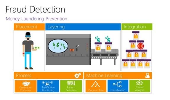
This was one of the use cases where Machine Learning plays a major role in improving the transactional business. One of the other usages of Machine Learning in Transactional Analytics is in Fraud Detection.
In this case, the system could understand patterns from the customer’s purchased data and predict the fraud in the new set of transactions based on the concept of cognitive computing. Machine Learning ensures the confidence level is high while deciding on a transaction. It also allows the evaluation of multiple transactions in real time.
With an increased number of transactions, the models tend to perform better. It maintains efficiency and often acts better than humans in dealing with fraudulent behaviors.
The fraud detection process starts with gathering the relevant data and perform exploratory data analysis on the data to get rid of noise from the data. It is then divided into training, testing, and validation data sets. Once the data set is ready, it is then fed to several classification algorithms like Logistic Regression, Decision Tree, Random Forest, and even neural networks which are fast and more efficient than conventional Machine Learning algorithms.
However, there are few drawbacks in Fraud Detection using Machine Learning such as Lack of inspectability, the possibility of overlooking some obvious activities like card sharing.
Machine Learning has a wide range of usage in the Transactional analytics and in this article we have seen a couple of such use cases. Dimensionless has several blogs and training to get started with Machine Learning and Data Science in general.
Follow this link, if you are looking to learn more about data science online!
There are a huge number of ML algorithms out there. Trying to classify them leads to the distinction being made in types of the training procedure, applications, the latest advances, and some of the standard algorithms used by ML scientists in their daily work. There is a lot to cover, and we shall proceed as given in the following listing:
Statistical Algorithms
Classification
Regression
Clustering
Dimensionality Reduction
Ensemble Algorithms
Deep Learning
Reinforcement Learning
AutoML (Bonus)
1. Statistical Algorithms
Statistics is necessary for every machine learning expert. Hypothesis testing and confidence intervals are some of the many statistical concepts to know if you are a data scientist. Here, we consider here the phenomenon of overfitting. Basically, overfitting occurs when an ML model learns so many features of the training data set that the generalization capacity of the model on the test set takes a toss. The tradeoff between performance and overfitting is well illustrated by the following illustration:
Overfitting – from Wikipedia
Here, the black curve represents the performance of a classifier that has appropriately classified the dataset into two categories. Obviously, training the classifier was stopped at the right time in this instance. The green curve indicates what happens when we allow the training of the classifier to ‘overlearn the features’ in the training set. What happens is that we get an accuracy of 100%, but we lose out on performance on the test set because the test set will have a feature boundary that is usually similar but definitely not the same as the training set. This will result in a high error level when the classifier for the green curve is presented with new data. How can we prevent this?
Cross-Validation
Cross-Validation is the killer technique used to avoid overfitting. How does it work? A visual representation of the k-fold cross-validation process is given below:
From Quora
The entire dataset is split into equal subsets and the model is trained on all possible combinations of training and testing subsets that are possible as shown in the image above. Finally, the average of all the models is combined. The advantage of this is that this method eliminates sampling error, prevents overfitting, and accounts for bias. There are further variations of cross-validation like non-exhaustive cross-validation and nested k-fold cross validation (shown above). For more on cross-validation, visit the following link.
There are many more statistical algorithms that a data scientist has to know. Some examples include the chi-squared test, the Student’s t-test, how to calculate confidence intervals, how to interpret p-values, advanced probability theory, and many more. For more, please visit the excellent article given below:
Classification refers to the process of categorizing data input as a member of a target class. An example could be that we can classify customers into low-income, medium-income, and high-income depending upon their spending activity over a financial year. This knowledge can help us tailor the ads shown to them accurately when they come online and maximises the chance of a conversion or a sale. There are various types of classification like binary classification, multi-class classification, and various other variants. It is perhaps the most well known and most common of all data science algorithm categories. The algorithms that can be used for classification include:
Logistic Regression
Support Vector Machines
Linear Discriminant Analysis
K-Nearest Neighbours
Decision Trees
Random Forests
and many more. A short illustration of a binary classification visualization is given below:
From openclassroom.stanford.edu
For more information on classification algorithms, refer to the following excellent links:
Regression is similar to classification, and many algorithms used are similar (e.g. random forests). The difference is that while classification categorizes a data point, regression predicts a continuous real-number value. So classification works with classes while regression works with real numbers. And yes – many algorithms can be used for both classification and regression. Hence the presence of logistic regression in both lists. Some of the common algorithms used for regression are
Linear Regression
Support Vector Regression
Logistic Regression
Ridge Regression
Partial Least-Squares Regression
Non-Linear Regression
For more on regression, I suggest that you visit the following link for an excellent article:
Both articles have a remarkably clear discussion of the statistical theory that you need to know to understand regression and apply it to non-linear problems. They also have source code in Python and R that you can use.
4. Clustering
Clustering is an unsupervised learning algorithm category that divides the data set into groups depending upon common characteristics or common properties. A good example would be grouping the data set instances into categories automatically, the process being used would be any of several algorithms that we shall soon list. For this reason, clustering is sometimes known as automatic classification. It is also a critical part of exploratory data analysis (EDA). Some of the algorithms commonly used for clustering are:
Hierarchical Clustering – Agglomerative
Hierarchical Clustering – Divisive
K-Means Clustering
K-Nearest Neighbours Clustering
EM (Expectation Maximization) Clustering
Principal Components Analysis Clustering (PCA)
An example of a common clustering problem visualization is given below:
From Wikipedia
The above visualization clearly contains three clusters.
Another excellent article on clustering refer the link
Dimensionality Reduction is an extremely important tool that should be completely clear and lucid for any serious data scientist. Dimensionality Reduction is also referred to as feature selection or feature extraction. This means that the principal variables of the data set that contains the highest covariance with the output data are extracted and the features/variables that are not important are ignored. It is an essential part of EDA (Exploratory Data Analysis) and is nearly always used in every moderately or highly difficult problem. The advantages of dimensionality reduction are (from Wikipedia):
It reduces the time and storage space required.
Removal of multi-collinearity improves the interpretation of the parameters of the machine learning model.
It becomes easier to visualize the data when reduced to very low dimensions such as 2D or 3D.
It avoids the curse of dimensionality.
The most commonly used algorithm for dimensionality reduction is Principal Components Analysis or PCA. While this is a linear model, it can be converted to a non-linear model through a kernel trick similar to that used in a Support Vector Machine, in which case the technique is known as Kernel PCA. Thus, the algorithms commonly used are:
Ensembling means combining multiple ML learners together into one pipeline so that the combination of all the weak learners makes an ML application with higher accuracy than each learner taken separately. Intuitively, this makes sense, since the disadvantages of using one model would be offset by combining it with another model that does not suffer from this disadvantage. There are various algorithms used in ensembling machine learning models. The three common techniques usually employed in practice are:
Simple/Weighted Average/Voting: Simplest one, just takes the vote of models in Classification and average in Regression.
Bagging: We train models (same algorithm) in parallel for random sub-samples of data-set with replacement. Eventually, take an average/vote of obtained results.
Boosting: In this models are trained sequentially, where (n)th model uses the output of (n-1)th model and works on the limitation of the previous model, the process stops when result stops improving.
Stacking: We combine two or more than two models using another machine learning algorithm.
(from Amardeep Chauhan on Medium.com)
In all four cases, the combination of the different models ends up having the better performance that one single learner. One particular ensembling technique that has done extremely well on data science competitions on Kaggle is the GBRT model or the Gradient Boosted Regression Tree model.
We include the source code from the scikit-learn module for Gradient Boosted Regression Trees since this is one of the most popular ML models which can be used in competitions like Kaggle, HackerRank, and TopCoder.
GradientBoostingClassifier supports both binary and multi-class classification. The following example shows how to fit a gradient boosting classifier with 100 decision stumps as weak learners:
GradientBoostingRegressor supports a number of different loss functions for regression which can be specified via the argument loss; the default loss function for regression is least squares ('ls').
import numpy as np
from sklearn.metrics import mean_squared_error
from sklearn.datasets import make_friedman1
from sklearn.ensemble import GradientBoostingRegressor

X, y = make_friedman1(n_samples=1200, random_state=0, noise=1.0)
X_train, X_test = X[:200], X[200:]
y_train, y_test = y[:200], y[200:]
est = GradientBoostingRegressor(n_estimators=100, learning_rate=0.1,
    max_depth=1, random_state=0, loss='ls').fit(X_train, y_train)
mean_squared_error(y_test, est.predict(X_test))
You can also refer to the following article which discusses Random Forests, which is a (rather basic) ensembling method.
In the last decade, there has been a renaissance of sorts within the Machine Learning community worldwide. Since 2002, neural networks research had struck a dead end as the networks of layers would get stuck in local minima in the non-linear hyperspace of the energy landscape of a three layer network. Many thought that neural networks had outlived their usefulness. However, starting with Geoffrey Hinton in 2006, researchers found that adding multiple layers of neurons to a neural network created an energy landscape of such high dimensionality that local minima were statistically shown to be extremely unlikely to occur in practice. Today, in 2019, more than a decade of innovation later, this method of adding addition hidden layers of neurons to a neural network is the classical practice of the field known as deep learning.
Deep Learning has truly taken the computing world by storm and has been applied to nearly every field of computation, with great success. Now with advances in Computer Vision, Image Processing, Reinforcement Learning, and Evolutionary Computation, we have marvellous feats of technology like self-driving cars and self-learning expert systems that perform enormously complex tasks like playing the game of Go (not to be confused with the Go programming language). The main reason these feats are possible is the success of deep learning and reinforcement learning (more on the latter given in the next section below). Some of the important algorithms and applications that data scientists have to be aware of in deep learning are:
Long Short term Memories (LSTMs) for Natural Language Processing
Recurrent Neural Networks (RNNs) for Speech Recognition
Convolutional Neural Networks (CNNs) for Image Processing
Deep Neural Networks (DNNs) for Image Recognition and Classification
Hybrid Architectures for Recommender Systems
Autoencoders (ANNs) for Bioinformatics, Wearables, and Healthcare
Deep Learning Networks typically have millions of neurons and hundreds of millions of connections between neurons. Training such networks is such a computationally intensive task that now companies are turning to the 1) Cloud Computing Systems and 2) Graphical Processing Unit (GPU) Parallel High-Performance Processing Systems for their computational needs. It is now common to find hundreds of GPUs operating in parallel to train ridiculously high dimensional neural networks for amazing applications like dreaming during sleep and computer artistry and artistic creativity pleasing to our aesthetic senses.
Artistic Image Created By A Deep Learning Network. From blog.kadenze.com.
For more on Deep Learning, please visit the following links:
In the recent past and the last three years in particular, reinforcement learning has become remarkably famous for a number of achievements in cognition that were earlier thought to be limited to humans. Basically put, reinforcement learning deals with the ability of a computer to teach itself. We have the idea of a reward vs. penalty approach. The computer is given a scenario and ‘rewarded’ with points for correct behaviour and ‘penalties’ are imposed for wrong behaviour. The computer is provided with a problem formulated as a Markov Decision Process, or MDP. Some basic types of Reinforcement Learning algorithms to be aware of are (some extracts from Wikipedia):
1.Q-Learning
Q-Learning is a model-free reinforcement learning algorithm. The goal of Q-learning is to learn a policy, which tells an agent what action to take under what circumstances. It does not require a model (hence the connotation “model-free”) of the environment, and it can handle problems with stochastic transitions and rewards, without requiring adaptations. For any finite Markov decision process (FMDP), Q-learning finds a policy that is optimal in the sense that it maximizes the expected value of the total reward over any and all successive steps, starting from the current state. Q-learning can identify an optimal action-selection policy for any given FMDP, given infinite exploration time and a partly-random policy. “Q” names the function that returns the reward used to provide the reinforcement and can be said to stand for the “quality” of an action taken in a given state.
2.SARSA
State–action–reward–state–action (SARSA) is an algorithm for learning a Markov decision process policy. This name simply reflects the fact that the main function for updating the Q-value depends on the current state of the agent “S1“, the action the agent chooses “A1“, the reward “R” the agent gets for choosing this action, the state “S2” that the agent enters after taking that action, and finally the next action “A2” the agent choose in its new state. The acronym for the quintuple (st, at, rt, st+1, at+1) is SARSA.
3.Deep Reinforcement Learning
This approach extends reinforcement learning by using a deep neural network and without explicitly designing the state space. The work on learning ATARI games by Google DeepMind increased attention to deep reinforcement learning or end-to-end reinforcement learning. Remarkably, the computer agent DeepMind has achieved levels of skill higher than humans at playing computer games. Even a complex game like DOTA 2 was won by a deep reinforcement learning network based upon DeepMind and OpenAI Gym environments that beat human players 3-2 in a tournament of best of five matches.
For more information, go through the following links:
If reinforcement learning was cutting edge data science, AutoML is bleeding edge data science. AutoML (Automated Machine Learning) is a remarkable project that is open source and available on GitHub at the following link that, remarkably, uses an algorithm and a data analysis approach to construct an end-to-end data science project that does data-preprocessing, algorithm selection,hyperparameter tuning, cross-validation and algorithm optimization to completely automate the ML process into the hands of a computer. Amazingly, what this means is that now computers can handle the ML expertise that was earlier in the hands of a few limited ML practitioners and AI experts.
AutoML has found its way into Google TensorFlow through AutoKeras, Microsoft CNTK, and Google Cloud Platform, Microsoft Azure, and Amazon Web Services (AWS). Currently it is a premiere paid model for even a moderately sized dataset and is free only for tiny datasets. However, one entire process might take one to two or more days to execute completely. But at least, now the computer AI industry has come full circle. We now have computers so complex that they are taking the machine learning process out of the hands of the humans and creating models that are significantly more accurate and faster than the ones created by human beings!
The basic algorithm used by AutoML is Network Architecture Search and its variants, given below:
Network Architecture Search (NAS)
PNAS (Progressive NAS)
ENAS (Efficient NAS)
The functioning of AutoML is given by the following diagram:
If you’ve stayed with me till now, congratulations; you have learnt a lot of information and cutting edge technology that you must read up on, much, much more. You could start with the links in this article, and of course, Google is your best friend as a Machine Learning Practitioner. Enjoy machine learning!


;" src="https://dimensionless.in/how-to-discover-and-classify-metadata-using-apache-atlas-on-amazon-emr/embed/#?secret=5ySnzA1FzV" data-secret="5ySnzA1FzV" width="600" height="338" title="“How to Discover and Classify Metadata using Apache Atlas on Amazon EMR” — DIMENSIONLESS TECHNOLOGIES PVT.LTD." frameborder="0" marginwidth="0" marginheight="0" scrolling="no"></iframe>)